Coupling from the past

Introduction

This is a follow-up to one of last month’s posts that contained some images of randomly-generated “lozenge tilings.” The focus here is not on the tilings themselves, but on the perfectly random sampling technique due to Propp and Wilson known as “coupling from the past” (see references below) that was used to generate them. As is often the case here, I don’t have any new mathematics to contribute; the objective of this post is just to go beyond the pseudo-code descriptions of the technique in most of the literature, and provide working Python code with a couple of different example applications.

The basic problem is this: suppose that we want to sample from some probability distribution over a finite discrete space , and that we have an ergodic Markov chain whose steady state distribution is . An approximate sampling procedure is to pick an arbitrary initial state, then just run the chain for some large number of iterations, with the final state as your sample. This idea has been discussed here before, in the context of card shuffling, the board game Monopoly, as well as the lozenge tilings from last month.

For example, consider shuffling a deck of cards using the following iterative procedure: select a random adjacent pair of cards, and flip a coin to decide whether to put them in ascending or descending order (assuming any convenient total ordering, e.g. first by rank, then by suit alphabetically). Repeat for some “large” number of iterations.

There are two problems with this approach:

1. It’s approximate; the longer we iterate the chain, the closer we get to the steady state distribution… but (usually) no matter when we stop, the distribution of the resulting state is never exactly .
2. How many iterations are enough? For many Markov chains, the mixing time may be difficult to analyze or even estimate.

Coupling from the past

Coupling from the past can be used to address both of these problems. For a surprisingly large class of applications, it is possible to sample exactly from the stationary distribution of a chain, by iterating multiple realizations of the chain until they are “coupled,” without needing to know ahead of time when to stop.

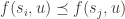
First, suppose that we can express the random state transition behavior of the chain using a fixed, deterministic function , so that for a random variable uniformly distributed on the unit interval,

In other words, given a current state and random draw , the next state is .

Now consider a single infinite sequence of random draws . We will use this same single source of randomness to iterate multiple realizations of the chain, one for each of the possible initial states… but starting in the past, and running forward to time zero. More precisely, let’s focus on two particular chains with different initial states and at time , so that

(Notice how the more random draws we generate, the farther back in time they are used. More on this shortly.)

A key observation is that if at any point, then the chains are “coupled:” since they experience the same sequence of randomness influencing their behavior, they will continue to move in lockstep for all subsequent iterations as well, up to . Furthermore, if the states at time zero are all the same for all possible initial states run forward from time , then the distribution of that final state is the stationary distribution of the chain.

But what if all initial states don’t end at the same final state? This is where the single source of randomness is key: we can simply look farther back in the past, say time steps instead of , by extending our sequence of random draws… as long as we re-use the existing random draws to make the same “updates” to the states at later times (i.e., closer to the end time zero).

Monotone coupling

So all we need to do to perfectly sample from the stationary distribution is

1. Choose a sufficiently large to look far enough into the past.
2. Run realizations of the chain, one for each initial state, all starting at time and running up to time zero.
3. As long as the final state is the same for all initial states, output as the sample. Otherwise, look farther back in the past (), generate additional random draws accordingly, and go back to step 2.

This doesn’t seem very helpful, since step 2 requires enumerating elements of the typically enormous state space. Fortunately, in many cases, including both lozenge tiling and card shuffling, it is possible to simplify the procedure by imposing a partial order on the state space– with minimum and maximum elements– that is preserved by the update function . That is, suppose that for all states and random draws , if , then .

Then instead of running the chain for all possible initial states, we can just run two chains, starting with the minimum and maximum elements in the partial order. If those two chains are coupled by time zero, then they will also “squeeze” any other initial state into the same coupling.

Following is the resulting Python implementation:

import random

def monotone_cftp(mc):
    """Return stationary distribution sample using monotone CFTP."""
    updates = [mc.random_update()]
    while True:
        s0, s1 = mc.min_max()
        for u in updates:
            s0.update(u)
            s1.update(u)
        if s0 == s1:
            break
        updates = [mc.random_update()
                   for k in range(len(updates) + 1)] + updates
    return s0

Sort of like the Fisher-Yates shuffle, this is one of those algorithms that is potentially easy to implement incorrectly. In particular, note that the list of “updates,” which is traversed in order during iteration of the two chains, is prepended with additional blocks of random draws as needed to start farther back in the past. The figure below shows the resulting behavior, mapping each output of the random number generator to the time at which it is used to update the chains.

Random draws in the order they are generated, vs. the order in which they are used in state transitions.

Coming back once again to the card shuffling example, the code below uses coupling from the past with random adjacent transpositions to generate an exactly uniform random permutation . (A similar example generating random lozenge tilings may be found at the usual location here.)

class Shuffle:
    def __init__(self, n, descending=False):
        self.p = list(range(n))
        if descending:
            self.p.reverse()

    def min_max(self):
        n = len(self.p)
        return Shuffle(n, False), Shuffle(n, True)

    def __eq__(self, other):
        return self.p == other.p

    def random_update(self):
        return (random.randint(0, len(self.p) - 2),
                random.randint(0, 1))

    def update(self, u):
        k, c = u
        if (c == 1) != (self.p[k] < self.p[k + 1]):
            self.p[k], self.p[k + 1] = self.p[k + 1], self.p[k]

print(monotone_cftp(Shuffle(52)).p)

The minimum and maximum elements of the partial order are the identity and reversal permutations, as might be expected; but it’s an interesting puzzle to determine the actual partial order that these random adjacent transpositions preserve. Consider, for example, a similar process where we select a random adjacent pair of cards, then flip a coin to decide whether to swap them or not (vs. whether to put them in ascending or descending order). This process has the same uniform stationary distribution, but won’t work when applied to monotone coupling from the past.

Re-generating vs. storing random draws

One final note: although the above implementation is relatively easy to read, it may be prohibitively expensive to store all of the random draws as they are generated. The slightly more complex implementation below is identical in output behavior, but is more space-efficient by only storing “markers” in the random stream, re-generating the draws themselves as needed when looking farther back into the past.

import random

def monotone_cftp(mc):
    """Return stationary distribution sample using monotone CFTP."""
    updates = [(random.getstate(), 1)]
    while True:
        s0, s1 = mc.min_max()
        rng_next = None
        for rng, steps in updates:
            random.setstate(rng)
            for t in range(steps):
                u = mc.random_update()
                s0.update(u)
                s1.update(u)
            if rng_next is None:
                rng_next = random.getstate()
        if s0 == s1:
            break
        updates.insert(0, (rng_next, 2 ** len(updates)))
    random.setstate(rng_next)
    return s0

 

References:

1. Propp, J. and Wilson, D., Exact Sampling with Coupled Markov Chains and Applications to Statistical Mechanics, Random Structures and Algorithms, 9 1996, p. 223-252 [PDF]
2. Wilson, D., Mixing times of lozenge tiling and card shuffling Markov chains, Annals of Applied Probability, 14(1) 2004, p. 274-325 [PDF]