Introduction
Consider the following problem: create a visually appealing digital image with exactly one pixel for each of the 16.8 million possible colors in the 24-bit RGB color space. Not a single color missing, and no color appearing more than once.
Check out the web site allRGB.com, which hosts dozens of such contributed images, illustrating all sorts of interesting approaches. Most of them involve coloring the pixels in some systematic way, although a few start with an existing image or photograph, and transform it so that it contains all possible colors, while still “looking like” the original image. I’ll come back to this latter idea later.
Hilbert’s curve
The motivation for this post is two algorithms that lend themselves naturally to this problem. The first is the generation of Hilbert‘s space-filling curve. The idea fascinated me when I first encountered it, in the May 1985 issue of the short-lived Enter magazine. How could the following code, that was so short, if indecipherable (by me, anyway), produce something so beautifully intricate?
 10 PI = 3.14159265: HCOLOR= 3
 20  HOME : VTAB 21
 30  PRINT "HILBERT'S CURVE."
 40  INPUT "WHAT SIZE? ";F1
 50  INPUT "WHAT LEVEL? ";L
 60  HGR
 70 PX = 0:PY =  - 60
 80 H = 0:P = 1
 90  GOSUB 110
 100  GOTO 20
 110  IF L = 0 THEN  RETURN
 120 L = L - 1:L1 = P * 90
 130 H = H + L1:P = ( - P)
 140  GOSUB 110
 150 P = ( - P)
 160  GOSUB 280
 170 R1 = P * 90:H = H - R1
 180  GOSUB 110
 190  GOSUB 280
 200  GOSUB 110
 210 R1 = P * 90:H = H - R1
 220  GOSUB 280
 230 P = ( - P)
 240  GOSUB 110
 250 P = ( - P):L1 = P * 90
 260 H = H + L1:L = L + 1
 270  RETURN
 280 HX =  COS (H * PI / 180)
 290 HY =  SIN (H * PI / 180)
 300 NX = PX + HX * F1
 310 NY = PY + HY * F1
 320  IF NX > 139 OR NY > 79 THEN GOTO 370
 330  HPLOT 140 + PX,80 - PY TO 140 + NX,80 - NY
 340 PX = NX:PY = NY
 350 PY = NY
 360  RETURN
 370  PRINT "DESIGN TOO LARGE"
 380  FOR I = 1 TO 1000: NEXT I
 390  GOTO 20
Nearly 30 years later, my first thought when encountering the allRGB problem was to use the Hilbert curve, but use it twice in parallel: traverse the pixels of the image via a 2-dimensional (order 12) Hilbert curve, while at the same time traversing the RGB color cube via a 3-dimensional (order 8) Hilbert curve, assigning each pixel in turn the corresponding color. The result looks like this (or see this video showing the image as it is constructed pixel-by-pixel):

allRGB image created by traversing image in 2D Hilbert curve order, assigning colors from the RGB cube in 3D Hilbert curve order.
(Aside: all of the images and videos shown here are reduced in size, using all 262,144 18-bit colors, for a more manageable 512×512-pixel image size.)
As usual and as expected, this was not a new idea. Aldo Cortesi provides an excellent detailed write-up and source code for creating a similar image, with a full-size submission on the allRGB site.
However, the mathematician in me prefers a slightly different implementation. Cortesi’s code is based on algorithms in the paper by Chris Hamilton and Andrew Rau-Chaplin (see Reference (2) below), in which the computation of a point on a Hilbert curve depends on both the dimension n (i.e., filling a square, cube, etc.) and the order (i.e., depth of recursion) of the curve. But we can remove this dependence on the order of the curve; it is possible to orient each successively larger-order curve so that it contains the smaller-order curves, effectively realizing a bijection between the non-negative integers 


The result is the following Python code, with methods Hilbert.encode() and Hilbert.decode() for converting indices to and from coordinates of points on the n-dimensional Hilbert curve:
class Hilbert:
    """Multi-dimensional Hilbert space-filling curve.
    """

    def __init__(self, n):
        """Create an n-dimensional Hilbert space-filling curve.
        """
        self.n = n
        self.mask = (1 << n) - 1

    def encode(self, index):
        """Convert index to coordinates of a point on the Hilbert curve.
        """

        # Compute base-n digits of index.
        digits = []
        while True:
            index, digit = divmod(index, self.mask + 1)
            digits.append(digit)
            if index == 0:
                break

        # Start with largest hypercube orientation that preserves
        # orientation of smaller order curves.
        vertex, edge = (0, -len(digits) % self.n)

        # Visit each base-n digit of index, most significant first.
        coords = [0] * self.n
        for digit in reversed(digits):

            # Compute position in current hypercube, distributing the n
            # bits across n coordinates.
            bits = self.subcube_encode(digit, vertex, edge)
            for bit in range(self.n):
                coords[bit] = (coords[bit] << 1) | (bits & 1)
                bits = bits >> 1

            # Compute orientation of next sub-cube.
            vertex, edge = self.rotate(digit, vertex, edge)
        return tuple(coords)

    def decode(self, coords):
        """Convert coordinates to index of a point on the Hilbert curve.
        """

        # Convert n m-bit coordinates to m base-n digits.
        coords = list(coords)
        m = self.log2(max(coords)) + 1
        digits = []
        for i in range(m):
            digit = 0
            for bit in range(self.n - 1, -1, -1):
                digit = (digit << 1) | (coords[bit] & 1)
                coords[bit] = coords[bit] >> 1
            digits.append(digit)

        # Start with largest hypercube orientation that preserves
        # orientation of smaller order curves.
        vertex, edge = (0, -m % self.n)

        # Visit each base-n digit, most significant first.
        index = 0
        for digit in reversed(digits):

            # Compute index of position in current hypercube.
            bits = self.subcube_decode(digit, vertex, edge)
            index = (index << self.n) | bits

            # Compute orientation of next sub-cube.
            vertex, edge = self.rotate(bits, vertex, edge)
        return index

    def subcube_encode(self, index, vertex, edge):
        h = self.gray_encode(index)
        h = (h << (edge + 1)) | (h >> (self.n - edge - 1))
        return (h & self.mask) ^ vertex

    def subcube_decode(self, code, vertex, edge):
        k = code ^ vertex
        k = (k >> (edge + 1)) | (k << (self.n - edge - 1))
        return self.gray_decode(k & self.mask)

    def rotate(self, index, vertex, edge):
        v = self.subcube_encode(max((index - 1) & ~1, 0), vertex, edge)
        w = self.subcube_encode(min((index + 1) | 1, self.mask), vertex, edge)
        return (v, self.log2(v ^ w))

    def gray_encode(self, index):
        return index ^ (index >> 1)

    def gray_decode(self, code):
        index = code
        while code > 0:
            code = code >> 1
            index = index ^ code
        return index

    def log2(self, x):
        y = 0
        while x > 1:
            x = x >> 1
            y = y + 1
        return y
[Edit: The FXT algorithm library contains an implementation of the multi-dimensional Hilbert curve, with an accompanying write-up whose example output suggests that it uses exactly this same convention.]
Random spanning trees
At this point, a key observation is that the Hilbert curve image above is really just a special case of a more general approach: we are taking a “walk” through the pixels of the image, and another “walk” through the colors of the RGB cube, in parallel, assigning colors to pixels accordingly. Those “walks” do not necessarily need to be along a Hilbert curve. In general, any pair of “reasonably continuous” paths might yield an interesting image.
A Hilbert curve is an example of a Hamiltonian path through the corresponding graph, where the pixels are vertices and adjacent pixels are next to each other horizontally or vertically. In general, Hamiltonian paths are hard to find, but in the case of the two- and three-dimensional grid graphs we are considering here, they are easier to come by. The arguably simplest example is a “serpentine” traversal of the pixels or colors (see Cortesi’s illustration referred to as “zigzag” order here), but the visual results are not very interesting. So, what else?
We’ll come back to Hamiltonian paths shortly. But first, consider a “less continuous” traversal of the pixels and/or colors: construct a random spanning tree of the grid graph, and traverse the vertices in… well, any of several natural orders, such as breadth-first, depth-first, etc.
So how to construct a random spanning tree of a graph? This is one of those algorithms that goes in the drawer labeled, “So cool because at first glance it seems like it has no business working as well as it does.”
First, pick a random starting vertex (this will be the root), and imagine taking a random walk on the graph, at each step choosing uniformly from among the current vertex’s neighbors. Whenever you move to a new vertex for the first time, “mark” or add the traversed edge to the tree. Once all vertices have been visited, the resulting marked edges form a spanning tree. That’s it. The cool part is that the resulting spanning tree has a uniform distribution among all possible trees.
But we can do even better. David Wilson (see Reference (3) below) describes the following improved algorithm that has the same uniform distribution on its output, but typically runs much faster: instead of taking a single meandering random walk to eventually “cover” all of the vertices, consider looping over the vertices, in any order, and for each vertex (that is not already in the tree) take a loop-erased random walk from that vertex until reaching the first vertex already in the tree. Add the vertices and edges in that walk to the tree, and repeat. Despite this “backward” growing of the tree, the resulting distribution is still uniform.
Here is the implementation in Python, where a graph is represented as a dictionary mapping vertices to lists of adjacent vertices:
import random

def random_spanning_tree(graph):
    """Return uniform random spanning tree of undirected graph.
    """
    root = random.choice(list(graph))
    parent = {root: None}
    tree = set([root])
    for vertex in graph:

        # Take random walk from a vertex to the tree.
        v = vertex
        while v not in tree:
            neighbor = random.choice(graph[v])
            parent[v] = neighbor
            v = neighbor

        # Erase any loops in the random walk.
        v = vertex
        while v not in tree:
            tree.add(v)
            v = parent[v]
    return parent
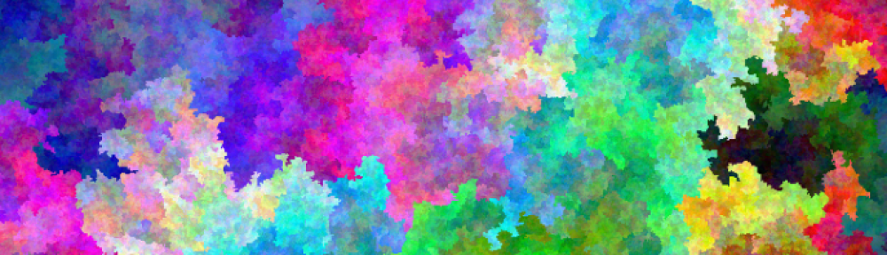
The following image shows one example of using this algorithm, visiting the image pixels in a breadth-first traversal of a random spanning tree, assigning colors according to a corresponding Hilbert curve traversal of the RGB color cube.

Breadth-first traversal of random spanning tree of pixels, assigning colors in Hilbert curve order.
My wife pointed out, correctly, I think, that watching the construction of these images is as interesting as the final result; this video shows another example of this same approach. Note how the animation appears to slow down, as the number of pixels at a given depth in the tree increases. A depth-first traversal, on the other hand, has a more constant speed, and a “snakier” look to it.
Expanding on this general idea, below is the result of all combinations of choices of four different types of paths through the image pixels and/or paths through the colors: Hilbert curve, serpentine, breadth-first through a random spanning tree, or depth-first.

Images resulting from different choices of paths through image pixels and colors.
Complete source code for generating larger versions of these images is available at the usual location here, in both Python, where I started, and C++, where I ended up, to manage the speed and space needed to create the full-size images.
Open questions
Let’s come back now to the earlier mention of (a) transforming an existing image to contain all possible colors, and (b) using Hamiltonian paths in some way. Reference (1) below describes a method of constructing a Hamiltonian cycle through the pixels of an image, using a minimum spanning tree of a “contraction” of the associated grid graph. The idea is to group the pixels into 2×2 square blocks of “mini-Hamiltonian-cycles,” resulting in a quarter-size grid graph, with edge weights between blocks corresponding to how “close” the pixel colors of the neighboring blocks are in the image.
Then, given a minimum spanning tree– or really, any spanning tree– in this smaller graph, we can construct a corresponding Hamiltonian cycle in the larger grid graph in a natural way, by connecting the 2×2 “mini-cycles” that are adjacent in the tree together into a larger cycle. The resulting Hamiltonian cycle tends to have pixels that are close together on the cycle be “close” in color as well.
Now consider the following allRGB image: start with an existing image, and construct a Hamiltonian cycle from the minimum-weight “block” spanning tree. Visit the pixels in cycle order, assigning colors according to some other corresponding “smooth” order, e.g. using a Hilbert curve. How much of the original image would still be apparent in the result?
References:
1. Dafner, R., Cohen-Or, D. and Matias, Y., Context-Based Space-Filling Curves, Eurographics 2000, 19:3 (2000) [PDF]
2. Hamilton, C. and Rau-Chaplin, A., Compact Hilbert Indices for Multi-Dimensional Data, Proceedings of the First International Conference on Complex, Intelligent and Software Intensive Systems, April 2007, 139-146 [PDF]
3. Wilson, D., Generating Random Spanning Trees More Quickly than the Cover Time, Proceedings of the 28th Annual ACM Symposium on the Theory of Computing, ACM (1996), 296-303 [PDF]

Very interesting and fun. I wonder if the results would be even more aesthetically pleasing if you somehow walked through CIELab space or X Y Z space.
Pingback: Hilbert halftone art | Possibly Wrong