Inverse Coupon Collector’s Problem

This is motivated by a recent blog post by John D. Cook [2] discussing the problem of estimating the number s of words in an author’s vocabulary, given an observation of the number k of distinct words in the author’s work of length n words.

The blog post references a paper by Brainerd [1], suggesting that it gives an estimate of s as the root of the following equation:

\sum\limits_{j=0}^{k-1}\frac{s}{s-j}=n

However, although Brainerd discusses several different estimation methods, I was unable to find any mention of this particular one, either explicitly or in derivation.

At any rate, the motivation for this post is simply to note that this is essentially the “inverse” of the coupon collector’s problem, discussed several times here before, which is usually stated in terms of expectation: if each purchased box of cereal contains one of s types of coupon, what is the expected number n of boxes we must purchase to obtain all s types of coupon?

This expected value is the above sum evaluated at k=s. More generally, even when k<s, the above sum is the expected number of boxes we must purchase to first observe k distinct coupon types. This suggests a nicely intuitive, although not rigorous, argument for using the above equation to solve the “inverse” problem: if we have observed k distinct coupon types among n purchased coupons, then a reasonable estimate for the unknown s is that value for which our number of observations n is the expected number of coupons needed to first observe k distinct types.

It’s interesting that this actually works. Sort of, anyway. That is, Dawkins [3] solves this inverse problem by computing the maximum likelihood estimate for s, which turns out to be one of the integer values on either side of the (generally non-integral) root of the equation above.

References:

  1. Brainerd, B., On the Relation between Types and Tokens in Literary Text, Journal of Applied Probability, 9(3) September 1972, p. 507-518 [JSTOR]
  2. Cook, John D., Estimating an author’s vocabulary [HTML]
  3. Dawkins, B., Siobhan’s Problem: The Coupon Collector Revisited, The American Statistician, 45(1) February 1991, p. 76-82 [JSTOR]

Lemonade Stand

This article was discussed on Hacker News.

Introduction

This was a fun nostalgia trip. But it ended up being an attempt to collect and preserve some retro computing history as well… and I also learned– or forgot and remembered?– another interesting quirk of that programming environment from nearly 45 years ago.

In 1981, I had a friend down the street who had an Apple II+. Later that year, my parents hired a tutor for programming lessons. I feel like I owe much of the subsequent course of my life to that time with “Mrs. Cathy,” who had several computers in her home: I remember an Apple II+, a VIC-20, and an IBM PC.

But it wasn’t until 1983 that we got our own home computer, an Apple //e. One of the programs that came with the computer, Lemonade Stand, is shown in the screenshot below.

The game is pretty simple: each morning, based on the weather forecast for the day, you decide how many glasses of lemonade and how many advertising signs to make, and how much to charge for each glass. These decisions and the day’s weather affect demand, you sell some number of glasses, rinse and repeat.

It’s about as fun as it sounds… but I remember being intrigued by the prospect of “reverse engineering” the game. The Applesoft BASIC source code contains the formula for computing the demand and the resulting profit as a function of the player’s inputs and the weather. We can, in principle, “solve” for the inputs that would maximize the expected profit. This post is motivated by my failed attempt to do this.

History

All of the code discussed here, both old and new, is available on GitHub. Let’s start with the old code: lemonade.bas is the Applesoft BASIC source by Charlie Kellner, from the .dsk image of my original 5.25″ diskette. I believe this is the earliest Apple version of the game– for completeness I’ve also included source extracts of two subsequent released versions (lemonade_v4.bas and lemonade_v5.bas), but for our purpose here their behavior is identical, with cosmetic updates to the graphics and sound by Drew Lynch, Bruce Tognazzini, and Jim Gerber.

For comparison, I’ve also extracted the source for selll.bas (as in “sell lemonade”), from the Minnesota Educational Computing Consortium (MECC, of Oregon Trail fame) Elementary Volume 3 disk A704. Although appearing later in 1980, I think this version is somewhat closer to the actual original version of the game written by Bob Jamison in 1973 for the UNIVAC mainframe. That original 1973 source seems to be lost to the mists of antiquity… but I think selll.bas retains more of its parentage than the Kellner version, which removed some helpful comments explaining the terms in the demand function, mistranslated some variable names and GOTO line numbering resulting in unreachable code, etc.

Maximizing profit

Now for the new code: lemonade_strategy.py implements the profit-maximization described above. It’s pure brute force: given the objective function below,

def expected_profit(glasses, signs, price, cost, r1=1, p_storm=0):
    n1 = 54 - 2.4 * price if price < 10 else 3000 / (price * price)
    demand = min(int(r1 * n1 * (2 - math.exp(-0.5 * signs))), glasses)
    revenue = demand * price
    expense = glasses * cost + signs * 15
    return ((1 - p_storm) * revenue - expense, revenue - expense,
            glasses, signs, price)

where r1 and p_storm are functions of the weather forecast, we simply evaluate the expected profit for all feasible inputs and find the maximum, with the wrinkle that the feasible region– how many glasses and signs we can possibly make– also depends on our current assets:

max(expected_profit(glasses, signs, price, cost, r1, p_storm)
    for glasses in range(min(1000, assets // cost) + 1)
    for signs in range(min(50, (assets - cost * glasses) // 15) + 1)
    for price in range(101))

I ended up in this rabbit hole in the usual way, after discussion with a student. My objective wasn’t really to “solve” this decades-old game, but just to give an explicit example of how much slower computers were then: this same brute-force approach in Applesoft BASIC, with the Apple //e’s 1 MHz processor, took nearly 4 hours to compute optimal strategy just for the first sunny day in Lemonsville. That’s over 200,000 times slower than the above Python code, which runs in a fraction of a second on my decade-old 2.6 GHz laptop– that is, with a clock speed “only” 2,600 times faster.

Changing the weather

You can play an Apple version of the game in a browser at the Internet Archive, linked from the game’s Wikipedia page. I did just that, with my Python script running alongside to compute optimal strategy… and it didn’t work.

The first day’s weather was “hot and dry.” With $2.00 and each glass of lemonade costing 2 cents, the optimal strategy should have been to make 74 glasses, 3 advertising signs, and charge 12 cents per glass, for an expected profit of $6.95. But when I entered these values in the game, I only sold 37 glasses, for a lousy $2.51 profit.

What was going on? It turns out that there are many different copies of Lemonade Stand out there, both at the Internet Archive as well as in various Apple II disk image archives… but the particular one linked from Wikipedia is unique among all of these in that it contains an important modification to the source code appearing in none of the other copies, highlighted below:

400  REM   WEATHER REPORT
410 SC = RND (1)
420 IF SC < .4 THEN SC = 2: GOTO 460
430 IF SC < .7 THEN SC = 10: GOTO 460
440 SC = 7
460 REM IF D<3 THEN SC=2

(You can play the original unmodified version at the Internet Archive here.)

I don’t know where these changes came from. And I believe these are indeed changes from the original release (i.e., not the other way around). But just these three edits were enough to keep my optimal strategy calculation from producing the correct result. This was strange at first glance, since the above section of code merely computes the randomly generated weather forecast for the day, which is an input to the subsequent profit calculation. In the above modified version, the weather forecast is sunny (SC=2) 40% of the time, cloudy (SC=10) 30% of the time, and hot and dry (SC=7) 30% of the time. The original threshold values are 0.6 and 0.8, corresponding to probabilities (0.6, 0.2, 0.2) of (sunny, cloudy, hot and dry).

The REM in line 460 is a “remark” comment, effectively disabling the original behavior of forcing sunny forecasts for the first two days (when D=1 and D=2) of the game. But again, why should this matter? This is all input to the profit calculation, which remains identical to the original, so what is causing the difference in behavior?

Undeclared variables

To make it easier to poke (!) around this problem, I wrote lemonade.py, which is my attempt at a shot-for-shot remake of the original lemonade.bas in Python, minus the graphics and sound– that is, just a canonical mode text interface, but an otherwise line-for-line direct translation with identical behavior.

That translation process was an interesting exercise, almost a logic puzzle, converting the unstructured GOTO-based flow control of Applesoft BASIC into structured Python– I was surprised at the end of it all to find that only a single defined function and extra temporary Boolean variable were needed, despite all of the GOSUBs.

That translation helped me to understand the cause of the different behavior I was seeing in the original. The problem is in the following section of code, with the offending lines highlighted:

700  REM   AFTER 2 DAYS THINGS CAN HAPPEN
710 IF D > 2 THEN 2000
...
2000 REM RANDOM EVENTS
2010 IF SC = 10 THEN 2110
2030 IF SC = 7 THEN 2410
...
2410 X4 = 1
2430 PRINT "A HEAT WAVE IS PREDICTED FOR TODAY!"
2440 R1 = 2
2450 GOTO 805

The variable R1 is an input to the profit function. But although the code change in line 460 above allows the first day’s displayed forecast to be hot and dry– or anything else other than sunny– line 710 still prevents actually setting R1 to reflect that non-sunny forecast when computing profit.

The effect is that, for the first two days, the weather forecast might indicate “hot and dry,” or “cloudy,” etc., but it’s really still sunny for those first two days, just like the original version.

All of which leads to the actual motivation for this post: when I initially tried to reproduce the effect of the three changed lines in the Python version, I got a “NameError: name 'D' is not defined“, due to commenting out line 460 in the BASIC version above: the variable D is never declared or assigned a value prior to line 460.

Python can’t handle this… but apparently Applesoft BASIC can. Variables do not need to be declared before use: when evaluating an expression containing a variable not previously assigned, the value of that variable defaults to zero (or the empty string for string variables).

This behavior is actually depended on in a few other places in the game as well. I admit that I think this is new to me– in all of those early days of learning programming, I don’t remember ever being aware of nor taking advantage of this “feature.” And it’s not a feature of the original Dartmouth BASIC. And I couldn’t find documentation of it anywhere in the books, manuals, and magazines that I have… but I did find it written down in the original “Blue Book” Applesoft Reference Manual. From page 9: “Another important fact is that if a variable is encountered in a formula before it is assigned a value, it is automatically assigned the value zero. Zero is then substituted as the value of the variable in the particular formula.

Exact analysis of Dreidel game

Introduction

A few weeks ago I read an interesting article by Hillel Wayne [6], discussed on Hacker News, describing analysis of Dreidel, a game traditionally played during the Jewish holiday of Hanukkah. Each player starts with the same number of tokens– often foil-wrapped chocolate coins– and antes one coin each into the center pot. Players take turns spinning the dreidel, with one of four equally likely outcomes:

  • Nun (“nothing”): player does nothing, turn passes to next player on the left.
  • Gimel (“everything”): player takes all of the coins in the pot. With the pot now empty, everyone, including the current player, antes one coin back into the pot.
  • Hei (“half”): player takes half of the coins in the pot. If there are an odd number of coins in the pot, the player rounds up, taking the larger half. If this empties the pot, i.e. if only one coin was in the pot, everyone– again including the current player– must ante one coin back into the pot.
  • Shin (“put”): player puts one coin into the pot.

A player is out of the game if they cannot put a coin into the pot when required. Play continues until one player remains, who wins all of the coins.

The motivation for this post is to try to improve upon past analyses of Dreidel, which involve various limitations, simplifying assumptions, and/or approximations in their solution; and to present exact probabilities and expected values for the game, that raise an interesting conjecture that appears to be new. The Python code is available on GitHub.

Another token-passing game

What initially caught my attention to this problem was how much it has in common with the Left-Center-Right dice game discussed in the previous post. Both Dreidel and Left-Center-Right are “games” with no strategy, with all “moves” dictated solely by the random outcome of a spin/roll. Both games involve passing tokens (coins) around among the players and a center pot, with the game ending with one player winning all of the coins.

We can thus apply essentially the same method to analyzing Dreidel, solving a sequence of linear systems of equations, indexing matrix rows and columns by ranking corresponding weak compositions of the coins in play… but with one modification. In Left-Center-Right, the number of players remains fixed throughout the game, but the number of coins in circulation is always decreasing; once a coin enters the pot, it stays there. In Dreidel, the opposite is true: all of the coins remain in circulation throughout the game, entering and leaving the pot, but the number of players decreases as players go “out” when they are unable to put a coin into the pot. Thus, in Dreidel the sequence of linear systems is indexed by the changing number of players, instead of by number of coins.

(As an aside, since I’m always on the lookout for nice exercises for students in mathematics or computer science: show that this same row/column indexing approach used in Left-Center-Right isn’t “wasteful” when applied to Dreidel. That is, show that every distribution of coins among the players, with a positive number of coins in the pot, is a reachable state of the game.)

Rule variations

Although this analysis assumes the specific rules of the game as described above, there are several variations supported in the Python code. For example, the article [6] that motivated this post seems unique in specifying min_coins=1, requiring players to always have a positive minimum number of coins, going out immediately if they ever have zero coins. We instead follow the convention assumed in all of the other references that min_coins=0: a player is only out when they can’t pay.

Another variation deals with taking half the pot when there are an odd number of coins. Robinson and Vijay [4] specify half_odd=0, rounding down, with the player taking the smaller half of the pot; but we follow the elsewhere-convention of half_odd=1, rounding up.

Results and conjecture

References [1] and [4] observe that Dreidel takes a long time to play, with a number of spins that varies (at most) quadratically as the number of players. The exact expected length of the game is shown in the figure below.

Expected number of turns (i.e., dreidel spins) and hours to complete a game, vs. number of coins each player starts with.

Assuming 8 seconds per spin as in [1], a four-player game would take almost 2 hours on average to complete if each player starts with 10 coins, and nearly 4.5 hours if each player starts with 15 coins.

What I found most interesting about Dreidel, however, is how the advantage varies with player position. All of the references below suggest that the first player to spin has an advantage (although based on simulation and/or various simplifying approximations), and that things get worse as we move around the table, with the last player to spin having the least probability of winning.

But if we compute these probabilities exactly, and present results as the expected return, or the average number of coins “gained” relative to initial wagered coins at the start of the game, we see the following interesting behavior:

Expected net coins won vs. number of starting coins wagered, for the starting player (blue) and for the last player (red).

I’ve sacrificed completeness to try to preserve clarity, only showing the first player’s return in blue, and the last player’s in red; the other players’ returns vary monotonically between these two extremes.

This figure suggests that a player’s expected return seems to very quickly approach a non-zero limit as the starting number of coins increases, that depends on the position of the player around the table. For example, in a game with four players, the first player to spin can expect to net about half a coin per game, no matter whether the players start with 2 coins each or 15, while the last player can expect to lose about half a coin per game.

References:

  1. Blatt, B., Dreidel: The classic Hannukah game is painfully slow. It’s time to speed it up, Slate, December 2014 [HTML]
  2. Feinerman, R., An Ancient Unfair Game, The American Mathematical Monthly, 83(8) October 1976, p. 623-625 [JSTOR]
  3. Lucas, S., Who wins when playing Dreidel, 2nd Mathematics Of Various Entertaining Subjects (MOVES) Conference, Museum of Mathematics, New York, August 2015 [PDF]
  4. Robinson, T. and Vijay, S., Dreidel lasts O(N^2) spins, Advances in Applied Mathematics, 36(1) January 2006, p. 85-94 [arXiv]
  5. Trachtenberg, F., The Game of Dreidel Made Fair, The College Mathematics Journal, 27(4) September 1996, p. 278-281 [JSTOR]
  6. Wayne, H., I formally modeled Dreidel for no good reason [HTML]

Analysis of Left-Center-Right dice game

Introduction

This game was surprisingly fun to play. Each player starts with three tokens– buttons or coins if you’re playing with kids, or dollar bills or even higher denominations if the adults want to make it more exciting. On each player’s turn, they roll one die for each of their tokens (up to a maximum of three dice rolled):

  • If a 1 is rolled, pass the token to the player’s left.
  • If a 2 is rolled, put the token in the “pot” in the center of the table.
  • If a 3 is rolled, pass the token to the player’s right.
  • If a 4, 5, or 6 is rolled, keep the token.

If a player has three or more tokens on their turn, only three dice are rolled. If a player has just one or two tokens, then they roll one or two dice, respectively. Most importantly, if a player has no tokens, they are not out of the game, since they might later receive tokens during a neighboring player’s turn; play simply passes to the next player with at least one token.

Play continues until only one player remains with any tokens. That player wins the game, collecting all of the tokens or bills or whatever, including those in the center pot.

I say “surprisingly fun” because, as was quickly observed during play, this is a “game” of pure chance. There is no skill involved; there are no decisions to be made. All of the token-passing game mechanics are merely a more time-consuming– but fun– way of randomly selecting which player will eventually win the game.

But that random selection isn’t quite uniform. Someone has to be the first player, the first to start risking loss of tokens, while the last player at the table gets to wait and watch. It’s an interesting problem to compute exactly how much effect playing order has on probability of winning.

Analysis results

The following table shows the exact probabilities (to given precision) of winning for each player, along with the expected number of turns to determine a winner, for games from two to seven players. (A turn is a roll of the dice, so that we do not count a turn for skipping a player without any tokens.) The Python code is available on GitHub.

# Players
234567
E(# turns)5.8098917.5158928.9454239.7020150.0633660.20762
Player
P(win)0.382070.306840.239260.193710.162120.139181
0.617930.328020.243180.193810.160990.137602
0.365140.255350.199940.164400.139523
0.262220.206320.169400.143174
0.206230.172620.146815
0.170470.148256
0.145467
Expected length of game and player win probabilities for each of up to 7 players, with lowest probability for a given number of players shown in red, highest probability in green.

The table layout is the same as this presentation of a Monte Carlo simulation analysis of the game. However, because those simulation results are only estimates, the order statistics indicated by red (lowest probability) and green (highest) are different in some places. For example, with five players, the first player, not the second, has the lowest probability of winning, and the next-to-last player has the greatest advantage.

These are close shaves– certainly close enough not to matter in a game played with children. But if this were a game played for money, then even these small differences in advantage are comparable to, for example, the magnitude of difference between an edge for the house or the player depending on minor variations in the rules for single-deck blackjack.

A sequence of linear systems

There were a few interesting implementation details. As discussed here before, we can compute the above probabilities (or expected values) as the solution of a system of linear equations. There is a variable x_{\mathbf{s},j} for each possible game state (\mathbf{s},j), where \mathbf{s} is a k-tuple indicating the number of tokens held by each of k players, and j \in \{0, 1, 2, \ldots, k-1\} is an integer indicating which player is to roll for the next turn.

Each variable x_{\mathbf{s},j} represents the probability of the first player winning the game (or the expected number of additional turns to complete the game), conditioned on the corresponding current game state (\mathbf{s}, j). That’s a lot of variables: k{4k \choose k} variables, which for k=7 players is already over 8 million variables.

But we don’t have to solve the entire system at once. The number of tokens in play never increases, so we can solve the very small subsystem involving only the game states with just one token in play, then use those cached results to construct and solve the subsystem of game states with two tokens in play, etc.

Ranking and unranking game states

To compute the resulting sparse matrix representing each of these linear systems, it is convenient to perfectly hash the game states to matrix row and column indices. In each game state, the tuple \mathbf{s} is a weak composition of the total number t \leq 3k of tokens remaining among the players (i.e., not in the center pot). Hashing weak compositions of t with k parts reduces to hashing k-1-subsets of \{1, 2, \ldots, t+k-1\}.

In most of the literature this process of perfect hashing from an object– in this case, a subset, or combination– to a consecutive integer index and back is referred to as ranking and unranking. We’ve done this before with permutations; for combinations, ranking is pretty straightforward:

def rank_subset(S, n=None):
    """Return colex rank of k-subset S of {0..n-1}."""
    return sum(math.comb(c, j + 1) for j, c in enumerate(S))

Note that this simple combinadic formula ranks subsets in colexicographic order. Lexicographic order take a bit more work, but in many applications such as this one, we just need an ordering, we don’t really care which one.

Unranking, or converting an integer index back to the corresponding subset, is the interesting subproblem that really motivated this post. Following is the basic guess-and-check algorithm:

def unrank_subset(r, n, k):
    """Return k-subset S of {0..n-1} with colex rank r."""
    S = [0] * k
    while k > 0:
        n = n - 1
        offset = math.comb(n, k)
        if r >= offset:
            r = r - offset
            k = k - 1
            S[k] = n
    return S

Those binomial coefficient calculations can be expensive, depending on the implementation, caching, etc. The following version implements the same basic algorithm, but takes advantage of the fact that the binomial coefficients needed at each iteration are “adjacent,” and thus differ by a simple factor:

def unrank_subset(r, n, k):
    """Return k-subset S of {0..n-1} with colex rank r."""
    S = [0] * k
    offset = math.comb(n, k)
    while k > 0:
        # Decrease n and update offset to comb(n, k).
        offset = offset * (n - k) // n
        n = n - 1
        if r >= offset:
            r = r - offset
            k = k - 1
            S[k] = n
            if k < n:
                offset = offset * (k + 1) // (n - k)
    return S

Finally, the following binary search version is generally worse than either of the above implementations when amortized over unranking of all possible subsets (as is needed in this game analysis), but it’s safer, so to speak, in that it still works in a reasonable amount of time even for astronomically large universal sets, i.e., when k \ll n.

def unrank_subset(r, n, k):
    """Return k-subset S of {0..n-1} with colex rank r."""
    S = [0] * k
    while k > 0:
        # Use binary search to decrease n until r >= comb(n, k).
        lower = k - 1
        while lower < n:
            mid = (lower + n + 1) // 2
            if r < math.comb(mid, k):
                n = mid - 1
            else:
                lower = mid
        r = r - math.comb(n, k)
        k = k - 1
        S[k] = n
    return S

But after all this, it’s worth acknowledging that none of this is strictly necessary for this particular problem. There is a space-time tradeoff to weigh here, where we could skip the ranking and unranking altogether, and simply pre-compute a dictionary mapping game states to array indices, via enumerate(itertools.combinations(...)) or any other convenient means of generating all states… that in this problem we have to store anyway to cache the probabilities (or expected values).

Counting Olympic medal podiums

From Rosen’s Discrete Mathematics and Its Applications textbook [1]:

Section 6.3 Exercise 47: There are six runners in the 100-yard dash. How many ways are there for three medals to be awarded if ties are possible? (The runner or runners who finish with the fastest time receive gold medals, the runner or runners who finish with exactly one runner ahead receive silver medals, and the runner or runners who finish with exactly two runners ahead receive bronze medals.)

I think it’s an interesting pedagogical question whether this is a “good problem” or not, at least in an academic setting. I think it could be a good problem… but like so many problems in combinatorics, this one generated quite a bit of confusion– justifiably, in my opinion– solely due to imprecise wording. Try it out for yourself: is the answer 260? Or 450? Or 873?

Before tackling this problem in more detail, I think it’s helpful to back up just a couple of exercises in the same section of the textbook, for a simpler and less ambiguous variant:

Section 6.3 Exercise 45: How many ways are there for a horse race with three horses to finish if ties are possible? [Note: Two or three horses may tie.]

With just three horses, an explicit case analysis isn’t too bad, and is perhaps the intended approach for students in an introductory course, without generating functions or other more heavyweight tools. But students are familiar with recurrence relations at this point, which yields a pretty elegant solution that also generalizes to compute the number b_n of race outcomes for any number n of horses:

b_n=\sum\limits_{k=1}^n {n \choose k}b_{n-k}, b_0=1

Coming back now to awarding medals to runners: although the parenthetical explanation of the rules above seems reasonably clear, the confusion arises in the possible conflict with the statement of the question itself. That is, are we counting only “podiums” where (a) exactly three medals are awarded, despite the rules allowing for more than three runners to receive medals in some cases of ties? Or are we perhaps counting podiums where (b) all three types of medal (gold, silver, and bronze) are awarded, possibly more than one of each type (although per the stated rules this would only ever involve multiple bronze medals, behind exactly one gold and one silver)?

Or are we simply counting podiums where (c) three or more medals are awarded, of three or fewer types, accounting for ties as explained in the subsequent description of the rules? This turns out to be the intended problem, with a modestly complex case analysis described in this top math.stackexchange.com answer… but trying to generalize to more than n=6 runners, or worse, to more than m=3 medal types (i.e., steps on the podium), seems daunting.

A recurrence relation can simplify the solution here as well, with a_{n,m} counting the number of such podiums:

a_{n,m}=\sum\limits_{k=1}^n {n \choose k}a_{n-k,m-k}

where a_{n,m}=1 if n \leq 0 or m \leq 0… or answering the other variants with the same recurrence, but with different initial conditions.

Finally, part of the motivation for this post was my lack of knowledge of how this has worked in actual events. Without the clarification in the problem statement, I thought that all runners with the fastest time would receive gold medals, and all runners with the second fastest time would receive silver, and all runners with the third fastest time would receive bronze. That hasn’t been the case at least in the Olympics, although there have been some isolated exceptions.

Reference:

  1. Rosen, K. H. (2019). Discrete Mathematics and Its Applications (8th ed.). New York, NY: McGraw-Hill. ISBN-13: 978-1-259-67651-2

Coupon collector’s problem variants with group drawings

Introduction

The coupon collector’s problem is an old standby in the puzzle community: what is the minimum number N of random selections with replacement from a set of s=1000 coupons that are needed to obtain at least one of every coupon in the set? This post collects solutions to some variants of this problem involving what Stadje [3] refers to as “group drawings,” where each random selection is not of a single coupon, but of a group of m=10 coupons. Python code implementing the formulas described here is available on GitHub.

Group drawing a subset (without replacement)

Results depend on how each group of coupons is selected. Stadje addresses the variant where at each turn we select a random subset of m distinct coupon types, i.e., sampling the m coupons without replacement (but always returning all coupons to the pile for the next turn).

In this case, the cumulative distribution function for N is

P(N \leq n)=\frac{1}{{s \choose m}^n}\sum\limits_{k=0}^{s} (-1)^k {s \choose k}{s-k \choose m}^n

with expected value

E(N)=-\sum\limits_{k=1}^{s} (-1)^k {s \choose k}\frac{1}{1-\frac{{s-k \choose m}}{{s \choose m}}}

Group drawing with replacement

Alternatively, we have considered here before the variant where at each turn we sample a group of m coupons with replacement, so that duplicates are possible within a group. In this case,

P(N \leq n)=\frac{1}{(s^m)^n}\sum\limits_{k=0}^{s} (-1)^k {s \choose k}(s-k)^{m n}

E(N)=-\sum\limits_{k=1}^{s} (-1)^k {s \choose k}\frac{1}{1-\frac{(s-k)^m}{s^m}}

Group drawing consecutively from a cycle

So far, nothing new. But this post was motivated by an interesting variant of the problem posed recently by John D. Cook [1]: arrange the s coupons in a circle, and at each turn, randomly select an “interval” of m coupons that appear consecutively around the circle.

A comment on the linked blog post mentions a very elegant solution to the continuous version of this problem described in [2,4,5], where we ask for the number N of random arcs of fixed length needed to cover the circle. For reference, the resulting distribution of N in this continuous case is given by

P(N \leq n)=\sum\limits_{k=0}^{\lfloor 1/a \rfloor} (-1)^k {n \choose k}(1-k a)^{n-1}

E(N)=1+\sum\limits_{k=1}^{\lfloor 1/a \rfloor} (-1)^{k-1}\frac{(1-k a)^{k-1}}{(k a)^{k+1}}

where a is the length of each arc as a fraction of the circumference.

It is a delightfully challenging exercise to apply this same inclusion-exclusion approach, where we are prohibiting uncovered “gaps” between arcs, to this discrete “consecutive coupon” collector problem. The resulting probability distribution is

P(N \leq n)=\frac{1}{s^n}\sum\limits_{j=1}^{n} \frac{s}{j} \left( \sum\limits_{k=0}^{j-1} (-1)^k {j \choose k}(j-k)^n \right) \left( \sum\limits_{k=0}^{\lfloor (s-j)/m \rfloor} (-1)^k {j \choose k}{s-1-k m \choose j-1} \right)

where the first inner summation counts ways to select exactly j specified distinct intervals in n turns (i.e., the number of surjections from [n] to [j]), and the second inner summation is the discrete analog to the continuous case summation above, counting ways to “cover” the entire cycle of s coupons with j distinct intervals of m consecutive coupons.

Unfortunately, unlike the other variants where we can compute the expected number of turns as a finite sum, it’s not clear to me how to compute the expected value here other than lower bound approximations from the series E(N)=\sum_{n=0}^{\infty}1-P(N<=n).

References:

  1. Cook, John D., Consecutive coupon collector problem [HTML]
  2. Solomon, H., Covering a Circle Circumference and a Sphere Surface, Chapter 4 in Geometric Probability, Philadelphia, PA: SIAM, p. 75-96, 1978 [PDF]
  3. Stadje, Wolfgang, The Collector’s Problem with Group Drawings, Advances in Applied Probability, 22(4) December 1990, p. 866-882 [JSTOR]
  4. Stevens, W. L., Solution to a Geometrical Problem in Probability, Annals of Eugenics, 9(4) 1939, p. 315-320 [PDF]
  5. Weisstein, Eric W., Circle Covering by Arcs, from MathWorld–A Wolfram Web Resource [HTML]

Angle interval intersection

Given two angle intervals, what is their intersection? An example of this problem is shown in the figure below.

Two open angle intervals, (30°,120°) in red, and (15°,75°) in blue, with their intersection (30°,75°) in purple.

Before we get to the solution, we need to make the problem more precise. But even before that, let’s start with a simpler problem whose solution will be a subroutine: computing the intersection of two real intervals on the number line. (I passed a milestone birthday recently, and I’m trying to lean into my age by using words like subroutine.)

Suppose that we have two such real intervals, each identified by their lower and upper bounds, A=(a_0,a_1) and B=(b_0,b_1). The following Python code computes their intersection as another interval:

def interval_intersect(a, b):
    """Intersection of two open intervals."""
    lower, upper = (max(a[0], b[0]), min(a[1], b[1]))
    return (min(lower, upper), upper)

Note that it is convenient to work with open intervals, excluding the endpoints, so that we won’t have to treat empty or degenerate intersections as a special case. (This does come at a cost of allowing multiple representations of the empty set, namely any interval with equal endpoints.)

Armed with this setup, we can now define an angle interval to be any open circular sector or arc… although I think using corresponding portions of an annulus in these visualizations does a better job than sectors or arcs of conveying the Venn-diagram-ness of the intersections we are trying to compute.

Just as we identify a real interval on the number line by its two endpoints, we can represent an angle interval by the two angles (a_0,a_1) made by its bounding radii relative to some zero reference… but we need some convention to deal with angle intervals that may contain that zero reference direction, as shown in the figure below.

Two open angle intervals, normalized (345°,405°) in red, and (30°,60°) in blue, with their unnormalized intersection (390°,405°), or normalized (30°,45°), in purple.

A convenient convention will be to enforce a_0 \leq a_1, so that the interval “sweeps counterclockwise” from direction a_0, through angle a_1-a_0, to direction a_1. And we can make such a representation unique if we “normalize” the bounding angles to enforce 0 \leq a_0 < 360^\circ (so that a_1 may exceed 360°; more on this shortly). The function below implements this normalization:

def normalize_angle_interval(a, circle=360):
    """Normalize open angle interval to lower bound in [0, circle)."""
    lower = a[0] % circle
    return (lower, lower + (a[1] - a[0]))

This convention greatly simplifies the case analysis involved in computing the intersection of two such normalized open angle intervals:

def angle_interval_intersect(a, b, circle=360):
    """Unnormalized intersection of normalized open angle intervals."""
    if a[1] > b[1]:
        b, a = a, b
    if a[0] + circle < b[1]:
        a = (a[0] + circle, a[1] + circle)
    return interval_intersect(a, b)

However, I’ve so far left out an important detail. The above implementation is correct, and reasonably elegant… as long as we are computing the intersection of open angle intervals that are not “wider” than 180°, such as the example shown in the figure below.

Two open angle intervals whose intersection is two disjoint intervals.

If we want to support intersections involving such “wide” angle intervals, then we have two problems: not only does the implementation become more complex, but even the interface does as well! That is, as the example above shows, in computing the intersection of two angle intervals we may need to return not just one but possibly two disjoint angle intervals.

In the application motivating this post, it was an acceptable tradeoff of generality for simplicity to restrict input angle intervals to at most 180°. And it’s a nice exercise to show that even if we allow “wide” inputs, the resulting single angle interval returned by the above implementation is either still correct, or at worst a subset of the full intersection.

East of here

This came up for a second time recently; during a family visit to the Assateague Island National Seashore, while standing on the beach looking east out over the Atlantic Ocean, it is natural to wonder, “What’s out there, beyond the horizon?”

There are at least two reasonable ways to make this question more precise. First, standing at a point somewhere on the east coast of North or South America, if we climb into our dinghy and row east… and continue to maintain an easterly heading throughout the trip, where do we first encounter land?

This is easy to plot on a world map with any cylindrical projection, since a constant east heading results in a track that is a horizontal line, as shown in the figure below.

Starting at Assateague Island in Maryland, rowing “ever east” brings us to the coast of Portugal.

But maintaining a constant east heading requires constantly turning (except at the equator). That is, if we imagine the oceans to be completely still water with no current, we must row with our left oar working harder than the right in order to maintain our east heading. Instead, suppose that we start rowing initially east, but continue rowing “ever straight” across the water, with both oars working equally hard, so that we are never locally turning. In this case, we are traveling along a geodesic, as shown in the figure below.

Again starting at Assateague Island, rowing initially east along a geodesic brings us to the disputed territory of Western Sahara on the coast of Africa.

The Python implementation of the geodesic direct and inverse problems (ported from the U.S. National Geodetic Survey Fortran source), as well as the map images (created using Natural Earth vector data version 5.1.1) and “coast to coast” example code used here are available on GitHub.

Grid search puzzle

In [3], Peter Winkler lists “seven problems you think you must not have heard correctly.” I think the following problem deserves to be on such a list:

Alice and Bob are playing a game, searching bins arranged in a grid with m=15 rows and n=30 columns, in which k=6 balls have been placed in distinct randomly selected bins. At each turn, both players simultaneously choose a bin to inspect. The first player to find a ball wins the game. (If both players choose the same bin containing a ball, the game ends in a draw.)

Alice decides to systematically search the grid row by row, left to right across each row, from the top row to the bottom. Bob decides to search columns, top to bottom, left to right. Which player is more likely to win? What if instead the game is played– using the same strategies above– on a slightly wider grid with n=31 columns? What if n=29?

I really like this problem, since a natural reaction might be, “How can either player possibly have an advantage?” (And for just k=1 ball, this intuition is correct; neither player has an advantage for any size grid.) While at the same time, it is an undergraduate-level problem to reasonably efficiently compute the exact probabilities of each player winning:

// Compute probability Alice wins by searching rows.
Rational p_grid_search_rows(int rows, int cols, int balls) {
    int ai = 1, aj = 0, bi = 0, bj = 0; // start in upper left
    Integer wins = 0;

    // Evaluate each bin/time where Alice finds a ball first.
    for (int bin = 1; bin <= rows * cols; ++bin) {
        if (++bi == rows) { bi = 0; ++bj; } // move Bob down
        if (bin < aj * rows + ai) { // verify Alice got here first

            // Place remaining balls in unsearched bins.
            int searched = 2 * bin - ai * bj - std::min(ai, bi);
            wins += binomial(rows * cols - searched, balls - 1);
        }
        if (++aj == cols) { aj = 0; ++ai; } // move Alice right
    }
    return Rational(wins, binomial(rows * cols, balls));
}

The result is that for the original problem with (m,n,k)=(15,30,6), Alice is at a very slight disadvantage, with an expected return E(A) on a unit wager of approximately -0.000274524, or -0.027%. But for most “wide” grids with more columns than rows, Alice has the advantage: intuitively, Alice spends more time exploring new territory, while Bob has to waste more turns on bins that Alice has already searched.
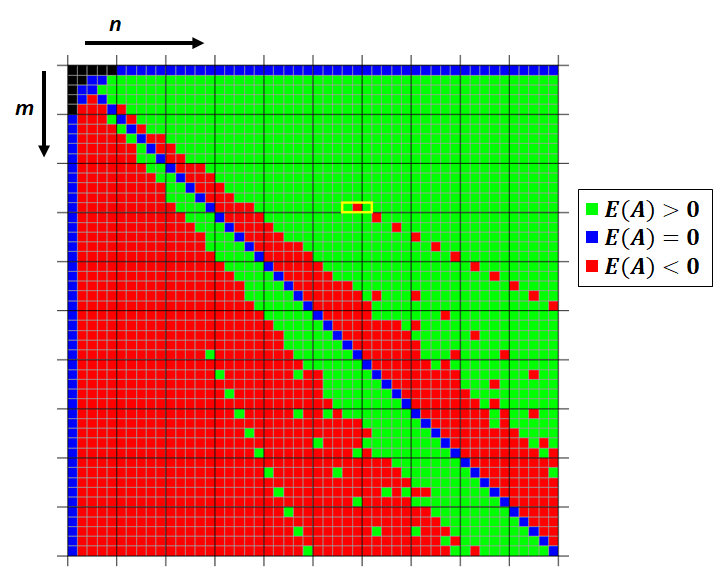
The figure below shows that it’s more complicated than this, though, indicating which player has the advantage as we vary the grid size, keeping the number of balls k=6 fixed (the three example grid sizes above are highlighted in yellow):

Figure shows which player has the advantage (green=Alice, red=Bob, blue=draw) as a function of grid size (m,n) with k=6 balls.

I first encountered this problem in [1] and [2], where the problem is generalized to consider search strategies as arbitrary permutations of the bins.

References:

  1. Chow, Timothy Y., Fair permutation problem and solution [PDF]
  2. Simons, Jim, solution 11523 in Problems and Solutions, The American Mathematical Monthly, 119(9) November 2012, p. 801-803 [JSTOR]
  3. Winkler, P., Seven Puzzles You Think You Must Not Have Heard Correctly, with solutions [PDF]

The pigeonhole principle: the converse is false

Introduction

I think the pigeonhole principle is the theorem that maximizes the ratio of “easy to state and prove” to “(not so) easy to apply to concrete problems.” The general theorem seems almost annoyingly obvious: if we put a greater number of pigeons into a fewer number of pigeonholes, then some pigeonhole must contain two or more pigeons. But in the context of a particular problem, it’s often difficult to see what objects are playing the roles of “pigeon” or “pigeonhole.”

But there are other potential pitfalls as well. The motivation for this post is to describe some of these other ways things can go wrong for students, using a particular common exercise as a running example.

Same subset sums

Consider the following problem: show that for any set S of k=10 positive integers each at most n=100, there exist two distinct subsets of S whose elements have the same sum. For example, given S=\{2,3,5,7,11,13,17,19,23,29\}, the subsets \{3,29\} and \{13,19\} both have the same sum of 32.

Here, the pigeons are the subsets of S, and the pigeonholes are the possible subset sums. There are 2^k=1024 subsets; how many possible sums are there? The empty set has sum zero, and the set \{91,92,93,94,95,96,97,98,99,100\} has the largest possible sum 955, for a total of

1+\frac{n(n+1)}{2}-\frac{(n-k)(n-k+1)}{2}

or 956 pigeonholes. If we put 1024 subsets into 956 pigeonholes labeled 0 to 955 according to their subset sum, then some pigeonhole must contain at least two pigeons, that is, there must exist two distinct subsets with the same sum.

The version of this problem at Cut-the-Knot asks for disjoint non-empty subsets with the same sum. It’s an exercise for the reader to show that this doesn’t really affect feasibility of the problem. However, the corresponding proof has an issue:

There are 1024 subsets of the 10 integers, but there can be only 901 (=955-55+1) possible sums, the number of integers between the minimum and maximum sums of ten distinct integers between 1 and 100. With more subsets than possible sums, there must exist at least one sum that corresponds to at least two subsets.

The argument here is that we only need 901 pigeonholes, labeled 55 through 955, since 55 is the minimum sum of the ten integers 1 through 10. But this is invalid, since it’s possible for some of our 1024 pigeons (subsets) to need to go into pigeonholes with labels (subset sums) that are less than 55, the empty set with sum zero being one extreme example.

This is tricky, since the logic here is wrong, but the conclusion is still true. To make the error more vivid, we need to consider a smaller version of the problem where the same invalid logic actually leads us to a false conclusion. Consider n=7 and k=4; then by the above reasoning, given any set S of 4 integers selected from \{1,2,3,4,5,6,7\}, there are 2^k=16 subsets of S, but only

\frac{n(n+1)}{2}-\frac{(n-k)(n-k+1)}{2}-\frac{k(k+1)}{2}+1

or 13 pigeonholes with labels from 1+2+3+4=10 to 4+5+6+7=22, suggesting that we should be able to find two distinct subsets of S with the same sum… and yet the set S=\{3,5,6,7\} is a counterexample, since all 16 of its subsets have distinct sums.

The converse is false

This problem has parameters (n,k) that we can vary. Let P(n,k) be the predicate asserting that every set S of k positive integers each at most n has distinct subsets with the same sum. Then we have seen above that P(100,10) is true, and that P(7,4) is false.

For another example, we can show that P(14,8) is true, using the pigeonhole principle as above: there are 2^8=256 possible subsets, and only 85 possible sums from zero to 7+8+9+10+11+12+13+14=84.

Can we make k smaller, and guarantee that smaller sets of integers still must have distinct subsets with the same sum? We can; the reader can verify that the pigeonhole argument works to show that P(14,7) is also true.

What about P(14,6)? Here, the same pigeonhole argument doesn’t work: there are only 2^6=64 pigeons, but 70 available pigeonholes with sum labels from zero to 9+10+11+12+13+14=69.

However, the pigeonhole inequality being false does not imply that the desired conclusion is also necessarily false. It turns out that P(14,6) is true; our pigeonhole argument is simply not sharp enough to show it.

This specific instance P(14,6) is a nice exercise to show that we can still use the pigeonhole principle here, but we need to be more careful about how many pigeonholes we really need. But even the linked solution is still imperfect, in the sense that this refined pigeonhole argument still does not characterize those parameter values for which P(n,k) is true. For example, the refined argument doesn’t work to show P(6,4), or P(9,5), etc.

This appears to remain an open problem; see OEIS sequences A201052 and A276661 for additional reading.