Counting marked dice

The following is from FiveThirtyEight.com’s Riddler:

I have an unlabeled, six-sided die. I make a single mark on the middle of each face that is parallel to one pair of that face’s four edges [see example in the figure below]. How many unique ways are there for me to mark the die? (Note: If two ways can be rotated so that they appear the same, then they are considered to be the same marking.)

Example marking of a die.

I think this is a particularly nice potential exercise for students for the usual reasons: on the one hand, wearing our mathematician hat, we can apply the lemma that is not Burnside’s… but this problem makes us think a bit harder about the coloring (i.e., how does each particular “color” represent an oriented mark on the die?), and about the distinction between the group of symmetries acting on the faces of the die versus the colorings of the faces of the die.

Alternatively, wearing our programmer hat, we can solve the problem (or maybe just verify our cocktail napkin approach above) by brute force enumeration of all possible markings, and count orbits under rotation with the standard trick of imposing some easy-to-implement ordering on the markings (converting each to its minimal representation under all possible rotations)… but again, what data structure should we use to represent a marking, that makes it easy to both enumerate all possibilities, and to compute orbits under rotation?

Following is my solution: we count the number of possible markings (“colorings”) that are fixed by each of the 24 rotational symmetries of the die, and average the results. To clarify the description of rotations, let’s temporarily distinguish one “red” face of the die, and group rotations according to the final location of the red face:

• If the red face stays in its original location, then:
  • The identity leaves all markings fixed.
  • Either of two quarter turns about the (axis normal to the) red face leaves zero markings fixed (since it changes the marking on the red face itself).
  • A half turn about the red face leaves markings fixed.
• If we rotate the red face a quarter turn to one of the four adjacent locations, then:
  • No additional rotation leaves zero markings fixed.
  • Either of two additional quarter turns about the (new axis normal to the) red face leaves markings fixed.
  • An additional half turn about the new red face leaves markings fixed.
• Finally, if we rotate the red face a half turn to the opposite face, then:
  • No additional rotation leaves markings fixed.
  • Either of two additional quarter turns about the new red face leaves markings fixed.
  • An additional half turn about the new red face leaves markings fixed.

Putting it all together, the number of distinguishable ways to mark the die is

All eight distinct ways to mark the die. Marks on opposing faces are the same color, with blue indicating parallel opposing marks, and red indicating skew (“perpendicular”) opposing marks.

The figure above shows the eight distinct ways to mark the die. Rather than “unfolding” the dice to explicitly show all six faces of each, the marks are colored red or blue, so that marks on opposing faces– one visible, one hidden– are the same color, with blue indicating parallel opposing marks, and red indicating skew, or “perpendicular,” opposing marks.

Analysis of horse racing board game

Introduction

I recently encountered a “horse racing” game played with two dice and a game board similar to the one shown in the figure below. Horses numbered 2 through 12 begin in the starting gate at the left, indicated by the green dots. At each turn, both dice are rolled yielding a total from 2 to 12, and the corresponding horse advances to the right one step, to the next black dot in their lane. The winner is the first horse to reach the finish line, indicated by the yellow dots.

Horse racing board game with the typical board layout.

What I found interesting about this game is the apparent intent to make the race fair. That is, for example, horse 7 is the most likely to advance on any particular dice roll, but this advantage is offset by requiring more steps to win. Indeed, if we describe the design of the board as a vector of integers indicating the required number of steps for each horse, in this case (3,6,8,11,14,17,14,11,8,6,3), then it makes at least some intuitive sense that these values are roughly in proportion to the corresponding dice probabilities.

However, this approach to leveling the playing field ends up being an extreme over-correction: horse 7 has way too far to go, winning the race less than 3% of the time, while Snake Eyes and Box Cars will each win over 19% of the time.

So, how can we fix this? Is there a better board design that more closely approximates a uniform distribution of wins across the eleven horses?

Scratching horses

First, I cheated a bit in the above description of the game. All eleven horses don’t actually race together; instead, before the race begins, the rules specify a procedure for scratching— i.e., removing from the race– four of the horses, and only the remaining seven horses race as described above. The scratching procedure is pretty simple: roll both dice, and scratch the corresponding horse. Continue rolling, ignoring rolls for horses that have already been scratched, until four distinct horses have been scratched. Similarly, during the race of the remaining seven horses, simply ignore any rolls for scratched horses. (I’m also leaving out the gambling nature of the game, which involves contributing chips or money to a winner-take-all pot with almost every dice roll; this scratching business really just serves to further increase the pot by stretching out the game a bit.)

To account for this, we need to compute the probability of scratching each of the C(11,4)=330 possible subsets of four horses, which we can then use to weight the probabilities of each of the unscratched horses subsequently winning the race.

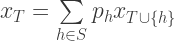
Given a particular subset of four horses, we compute the probability of exactly that subset being scratched by solving for in the linear system of equations in variables, indexed by subsets of , where

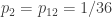
where is the single-roll probability of advancing horse (e.g., , etc.). In Python with SymPy (all code is available on GitHub):

def p_scratch(q):
    """Probability of scratching subset with dice probabilities q[:]."""
    a = sympy.eye(2 ** len(q))
    for i in range(2 ** len(q) - 1):
        for h, p_roll in enumerate(q):
            j = i | (2 ** h)
            a[i, j] -= p_roll
    return sympy.linsolve((a, sympy.eye(2 ** len(q))[:, -1])).args[0][0]

Win probabilities

At this point, given a particular subset of seven unscratched horses in a race, we are prepared to compute the probabilities of each of those horses winning, with a relatively simple modification of the generating function approach described in this earlier post, as the sum of coefficients for horse , where

and is the number of steps required for horse to win. Again in Python with NumPy (and the fractions module in case we want exact results):

def p_win1(p, n):
    """Probability of first horse winning."""
    g1 = P.polypow([Fraction(0), p[0]], n[0] - 1) / np.math.factorial(n[0] - 1)
    g2 = reduce(P.polymul,
                ([pi ** k / np.math.factorial(k) for k in range(ni)]
                 for pi, ni in zip(p[1:], n[1:])))
    g = reduce(P.polymul, [[p[0]], g1, g2])
    return sum(c * np.math.factorial(m) for m, c in enumerate(g))

Putting it all together, computing the overall probabilities of each horse winning the race after scratching four of the horses, it turns out that the scratching just makes the non-uniformity even worse, although only slightly: horse 7 now wins less than 2.5% of the time, and horses 2 and 12 win over 20% of the time.

Evaluating all board designs

So, finally, we can turn the above crank on each of the C(17+6-1,6)=74,613 different possible “reasonable” board designs, where by “reasonable” I mean symmetric (horses like 2 and 12 with the same dice probability should require the same number of steps to win) and monotonic (a horse like 7 with higher dice probability should never require fewer steps to win), ranging from the simplest first-roll-wins board (1,1,1,1,1,1,1,1,1,1,1) to the longest-race-but-still-unfair board (17,17,17,17,17,17,17,17,17,17,17). The figures below show some of the best results.

Probabilities of each horse 2-12 winning a race on various board designs (see colors below): at left, scratching no horses so that all 11 horses race; at right, scratching 4 horses and racing the remaining 7.

As already discussed, the original game board (3,6,8,11,14,17,14,11,8,6,3) fares pretty poorly. Interestingly, if we ignore scratching and just race all eleven horses together (figure at left), then the fairest board is pretty unambiguously (2,3,4,5,6,7,6,5,4,3,2)— almost but not quite the same as this Canadian version of the game– which minimizes all three of the norm (proportional to total variation distance), the norm, and the relative entropy distances from the uniform distribution.

If we play the standard game with four scratched horses (figure at right), then there are a few options depending on the yardstick for fairness. The board (4,7,9,11,13,15,13,11,9,7,4) minimizes the norm, and comes in third for the other two measures. The board (4,6,8,10,12,13,12,10,8,6,4) minimizes the norm and relative entropy, and comes in second for the norm. Alternatively, the board (4,6,8,10,12,14,12,10,8,6,4) comes in second, for both the no-scratch and four-scratch variants of the game, and for all three measures… except for the four-scratch norm, where it comes in fifth out of all candidate boards.