Distribution and variance in blackjack

Introduction

Analysis of casino blackjack has been a recurring passion project of mine for nearly two decades now.  I have been back at it again for the last couple of months, this time working on computing the distribution (and thus also the variance) of the outcome of a round.  This post summarizes the initial results of that effort.  For reference up front, all updated source code is available here, with pre-compiled binaries for Windows in the usual location here.

Up to this point, the focus has been on accurate and efficient calculation of exact expected value (EV) of the outcome of a round, for arbitrary shoe compositions and playing strategies, most recently including index play using a specified card counting system.  This is sufficient for evaluating playing efficiency: that is, how close to “perfect play” (in the EV-maximizing sense) can be achieved solely by varying playing strategy?

But advantage players do not just vary playing strategy, they also– and arguably more importantly– have a betting strategy, wagering more when they perceive the shoe to be favorable, wagering less or not at all when the shoe is unfavorable.  So a natural next step is to evaluate such betting strategies… but to do so requires not just expected value, but also the variance of the outcome of each round.  This post describes the software updates for computing not just the variance, but the entire probability distribution of possible outcomes of a round of blackjack.

Rules of the game

For consistency in all discussion, examples, and figures, I will assume the following setup: 6 decks dealt to 75% penetration, dealer stands on soft 17, doubling down is allowed on any two cards including after splitting pairs, no surrender… and pairs may be split only once (i.e., to a maximum of two hands).  Note that this is almost exactly the same setup as the earlier analysis of card counting playing efficiency, with the exception of not re-splitting pairs: although we can efficiently compute exact expected values even when re-splitting pairs is allowed, computing the distribution in that case appears to be much harder.

Specifying (vs. optimizing) strategy

The distribution of outcomes of a round depends on not only the rule variations as described above, but also the playing strategy.  This is specified using the same interface as the original interface for computing expected value, which looks like this:

virtual int BJStrategy::getOption(const BJHand & hand, int upCard,
                    bool doubleDown, bool split, bool surrender);

The method parameters specify the “zero memory” information available to the player: the cards in the current hand, the dealer’s up card, and whether doubling down, splitting, or surrender is allowed in the current situation.  The return value indicates the action the player should take: whether to stand, hit, double down, split, or surrender.  For example, the following implementation realizes the simple– but poorly performing– “mimic the dealer” strategy:

virtual int getOption(const BJHand & hand, int upCard,
        bool doubleDown, bool split, bool surrender) {
    if (hand.getCount() < 17) {
        return BJ_HIT;
    } else {
        return BJ_STAND;
    }
}

When computing EV, instead of returning an explicit action, we can also return the code BJ_MAX_VALUE, meaning, “Take whatever action maximizes EV in this situation.”  For example, the default base class implementation of BJStrategy::getOption() always returns BJ_MAX_VALUE, meaning, “Compute optimal composition-dependent zero memory (CDZ-) strategy, maximizing overall EV for the current shoe.”

However, handling this special return value requires evaluating all possible subsequent hands that may result (i.e., from hitting, doubling down, splitting, etc.).  When only computing EV, we can do this efficiently, but for computing the distribution, an explicit specification of playing strategy is required.

The figure below shows a comparison of the resulting distribution of outcomes for these two example strategies.

Probability distribution of player outcomes of a unit wager on a single round from a full shoe, using “mimic the dealer” strategy (red) vs. optimal strategy (blue).

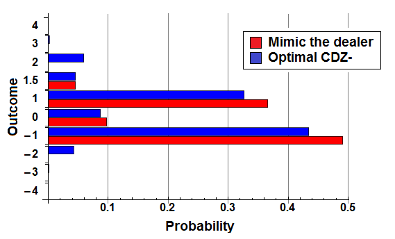
It is perhaps not obvious from this figure just how much worse “mimic the dealer” performs, yielding a house edge of 5.68% of initial wager; compare this with the house edge of just 0.457% for optimal CDZ- strategy.

Algorithm details

Blackjack is hard (i.e., interesting) because of splitting pairs.  It is manageably hard in the case of expected value, because expected value is linear: that is, if and are random variables indicating the outcome of the two “halves” of a split pair, then the expected value of the overall outcome, , is simply the sum of the individual expected values, .  Better yet, when both halves of the split are resolved using the same playing strategy, those individual expected values are equal, so that we need only compute .  (When pairs may be split and re-split, things get slightly more complicated, but the idea still applies.)

Variance, on the other hand, is not linear– at least when the summands are correlated, which they certainly are in the case of blackjack split hands.  So my first thought was to simply try brute force, recursively visiting all possible resolutions of a round.  Weighting each resulting outcome by its probability of occurrence, we can compute not just the variance, but the entire distribution of the outcome of the round.

This was unacceptably slow, taking about 5 minutes on my laptop to compute the distribution for CDZ- strategy from a full 6-deck shoe.  (Compare this with less than a tenth of a second to compute the CDZ- strategy itself and the corresponding overall EV.)  It was also not terribly accurate: the “direct” computation of overall EV provides a handy source of ground truth against which we can compare the “derived” overall EV using the distribution.  Because computing that distribution involved adding up over half a billion individual possible outcomes of a round, numerical error resulted in loss of nearly half of the digits of double precision.  A simple implementation of Kahan’s summation algorithm cleaned things up.

Two modifications to this initial approach resulted in a roughly 200-fold speedup, so that the current implementation now takes about 2.5 seconds to compute the distribution for the same full 6-deck optimal strategy.  First, the Steiner tree problem of efficiently calculating the probabilities of outcomes of the dealer’s hand can be split up into 10 individual trees, one for each possible up card.  This was an interesting trade-off: when you know you need all possible up cards for all possible player hands– as in the case of computing overall EV– there are savings to be gained by doing the computation for all 10 up cards at once.  But when computing the distribution, some player hands are only ever reached with some dealer up cards, so there is benefit in only doing the computation for those that you need… even if doing them separately actually makes some of that computation redundant.

Second, and most importantly, we don’t have to recursively evaluate every possible resolution of pair split hands.  The key observation is that (1) both halves of the split have the same set of possible hands– viewed as unordered subsets of cards– that may result; and (2) each possible selection of pairs of such resolved split hands may occur many times, but each with the same probability.  So we need only recursively traverse one half of any particular split hand, recording the number of times we visit each resolved hand subset.  Then we traverse the outer product of pairs of such hands, computing the overall outcome and “individual” probability of occurrence, multiplied by the number of orderings of cards that yield that pair of hands.

3:2 Blackjack isn’t always optimal

Finally, I found an interesting, uh, “feature,” in my original implementation of CDZ- strategy calculation.  In early testing of the distribution calculation, I noticed that the original direct computation of overall EV didn’t always agree with the EV derived from the computed distribution.  The problem turned out to be the “special” nature of a player blackjack, that is, drawing an initial hand of ten-ace, which pays 3:2 (when the dealer does not also have blackjack).

There are extreme cases where “standing” on blackjack is not actually optimal: for example, consider a depleted shoe with just a single ace and a bunch of tens.  If you are dealt blackjack, then you can do better than an EV of 1.5 from the blackjack payoff, by instead doubling down, guaranteeing a payoff of 2.0.  Although interesting, so far no big deal; the previous and current implementations both handle this situation correctly.

But now suppose that you are initially dealt a pair of tens, and optimal strategy is to split the pair, and you subsequently draw an ace to one of those split hands.  This hand does not pay 3:2 like a “normal” blackjack… but deciding what “zero memory” action to take may depend on when we correct the expected value of standing on ten-ace to its pre-split 3:2 payoff: in the previous implementation, this was done after the post-split EVs were computed, meaning that the effective strategy might be to double down on ten-ace after a split, but stand with the special 3:2 payoff on an “actual” blackjack.

Since this violates the zero memory constraint of CDZ-, the current updated implementation performs this correction before post-split EVs are computed, so that the ten-ace playing decision will be the same in both cases.  (Note that the strategy calculator also supports the more complex CDP1 and CDP strategies as well, the distinctions of which are for another discussion.)

What I found interesting was just how common this seemingly pathological situation is.  In a simulation of 100,000 shoes played to 75% penetration, roughly 14.5% of them involved depleted shoe compositions where optimal strategy after splitting tens and drawing an ace was to double down instead of stand.  As expected, these situations invariably occurred very close to the cut card, with depleted shoes still overly rich in tens.  (For one specific example, consider the shoe represented by the tuple (6, 6, 1, 5, 8, 2, 5, 9, 2, 34), indicating 6 aces, 6 twos, 34 tens, etc.)

Wrapping up, this post really just captures my notes on the assumptions and implementation details of the computation of the probability distribution of outcomes of a round of blackjack.  The next step is to look at some actual data, where one issue I want to focus on is a comparison of analysis approaches– combinatorial analysis (CA) and Monte Carlo simulation– their relative merits, and in particular, the benefits of combining the two approaches where appropriate.