Guess the number

I haven’t posted a puzzle in a while.  The following problem has the usual nice characteristics; it works on a cocktail napkin or as a programming problem, via exact solution or simulation, etc.

I am thinking of a randomly selected integer between 1 and (inclusive).  You are the first of players who will each, in turn, get a single guess at the selected number.  The player whose guess is closest wins $300, with ties splitting the winnings evenly.

Here is the catch: each player may not guess a number that has already been guessed by a previous player.  As the first player, what should your strategy be?  Which player, if any, has the advantage?  And what happens if we vary and ?

Probability of a Scrabble bingo

My wife and I have been playing Scrabble recently.  She is much better at the game than I am, which seems to be the case with most games we play.  But neither of us are experts, so that bingos— playing all 7 tiles from the rack in a single turn, for a 50-point bonus– are rare.  I wondered just how rare they should be… accounting for the fact that I am a novice player?

Let’s focus the problem a bit, and just consider the first turn of the game, when there are no other tiles on the board: what is the probability that 7 randomly drawn Scrabble tiles may be played to form a valid 7-letter word?

There are , or over 16 billion equally likely ways to draw a rack of 7 tiles from the 100 tiles in the North American version of the game.  But since some tiles are duplicated, there are only 3,199,724 distinct possible racks (not necessarily equally likely).  Which of these racks form valid words?

It depends on what we mean by valid.  According to the 2014 Official Tournament and Club Word List (the latest for which an electronic version is accessible), there are 25,257 playable words with 7 letters… but many of those are words that I don’t even know, let alone expect to be able to recognize from a scrambled rack of tiles.  We need a way to reduce this over-long official list of words down to a “novice” list of words– or better yet, rank the entire list from “easiest” to “hardest,” and compute the desired probability as a function of the size of the accepted dictionary.

The Google Books Ngrams data set (English version 20120701) provides a means of doing this.  As we have done before (described here and here), we can map each 7-letter Scrabble word to its frequency of occurrence in the Google Books corpus, the idea being that “easier” words occur more frequently than “harder” words.

The following figure shows the sorted number of occurrences of all 7-letter Scrabble words on a logarithmic scale, with some highlighted examples, ranging from between, the single most frequently occurring 7-letter Scrabble word, to simioid, one of the least frequently occurring words… and this doesn’t even include the 1444 playable words– about 5.7% of the total– that appear nowhere in the entire corpus, such as abaxile and zygoses.

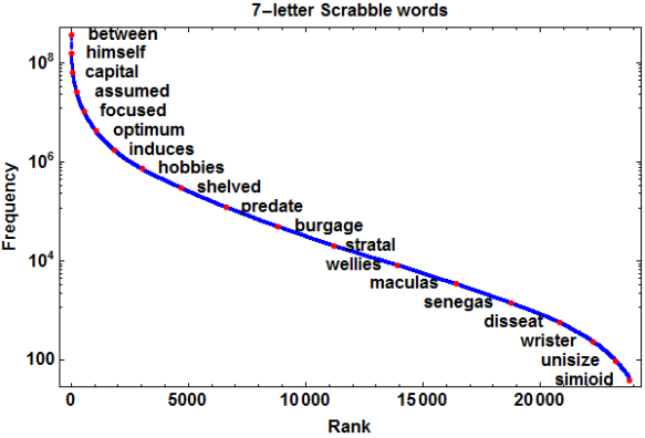
Scrabble 7-letter words ranked by frequency of occurrence in Google Books Ngrams data set.  The least frequent word shown here that I recognize is “predate.”

Armed with this sorted list of 25,257 words, we can now compute, as a function of , the probability that a randomly drawn rack of 7 tiles may be played to form one of the easiest words in the list.  Following is Mathematica code to compute these probabilities.  This would be slightly simpler– and much more efficient– if not for the wrinkle of dealing with blank tiles, which allow multiple different words to be played from the same rack of tiles.

tiles = {" " -> 2, "a" -> 9, "b" -> 2, "c" -> 2, "d" -> 4, "e" -> 12,
   "f" -> 2, "g" -> 3, "h" -> 2, "i" -> 9, "j" -> 1, "k" -> 1, "l" -> 4,
   "m" -> 2, "n" -> 6, "o" -> 8, "p" -> 2, "q" -> 1, "r" -> 6, "s" -> 4,
   "t" -> 6, "u" -> 4, "v" -> 2, "w" -> 2, "x" -> 1, "y" -> 2, "z" -> 1};

{numBlanks, numTiles} = {" " /. tiles, Total[Last /@ tiles]};

racks[w_String] := Map[
  StringJoin@Sort@Characters@StringReplacePart[w, " ", #] &,
  Map[{#, #} &, Subsets[Range[7], numBlanks], {2}]]

draws[r_String] :=
 Times @@ Binomial @@ Transpose[Tally@Characters[r] /. tiles]

all = {};
p = Accumulate@Map[(
       new = Complement[racks[#], all];
       all = Join[all, new];
       Total[draws /@ new]
       ) &,
     words] / Binomial[numTiles, 7];

The results are shown in the following figure, along with another sampling of specific playable words.  For example, if we include the entire official word list, the probability of drawing a playable 7-letter word is 21226189/160075608, or about 0.132601.

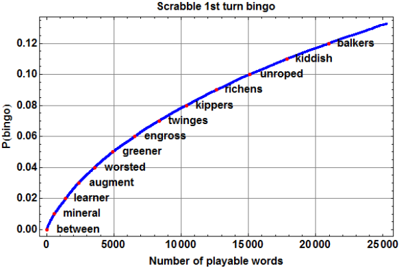
Probability that 7 randomly drawn tiles form a word, vs. dictionary size.

A coarse inspection of the list suggests that I confidently recognize only about 8 or 9 thousand– roughly a third– of the available words, meaning that my probability of playing all 7 of my tiles on the first turn is only about 0.07.  In other words, instead of a first-turn bingo every 7.5 games or so on average, I should expect to have to wait nearly twice as long.  We’ll see if I’m even that good.

Risk of (gambler’s) ruin

Suppose that you start with an initial bankroll of dollars, and repeatedly make a wager that pays $1 with probability , and loses $1 with probability .  What is the risk of ruin, i.e., the probability that you will eventually go broke?

This is the so-called gambler’s ruin problem.  It is a relatively common exercise to show that if , the probability of ruin is 1, and if , then the probability is

But what if the wager is not just win-or-lose a dollar, but is instead specified by an arbitrary probability distribution of outcomes?  For example, suppose that at each iteration, we may win any of units, with respective probabilities .  The purpose of this post is to capture my notes on some seemingly less well-known results in this more general case.

(The application to my current study of blackjack betting is clear: we have shown that, at least for a shoe game, even if we play perfectly, we are still going to lose if we don’t vary our bet.  We can increase our win rate by betting more in favorable situations… but a natural constraint is to limit our risk of ruin, or probability of going broke.)

Schlesinger (see Reference (2) below) gives the following formula for risk of ruin, due to “George C., published on p. 8 of ‘How to Win $1 Million Playing Casino Blackjack'”:

where and are the mean and standard deviation, respectively, of the outcome of each round (or hourly winnings).  It is worth emphasizing, since it was unclear to me from the text, that this formula is an approximation, albeit a pretty good one.  The derivation is not given, but the approach is simple to describe: normalize the units of both bankroll and outcome of rounds to have unit variance (i.e., divide everything by ), then use the standard two-outcome ruin probability formula above with win probability chosen to reflect the appropriate expected value of the round, i.e., .

The unstated assumption is that (note that ruin is guaranteed if , or if and ), and that accuracy of the approximation depends on , which is fortunately generally the case in blackjack.

There is an exact formula for risk of ruin, at least as long as outcomes of each round are bounded and integral.  In Reference (1) below, Katriel describes a formula involving the roots inside the complex unit disk of the equation

where is the probability of winning units in each round.  Execution time and numeric stability make effective implementation tricky.

Finally, just to have some data to go along with the equations, following is an example of applying these ideas to analysis of optimal betting in blackjack.  Considering the same rules and setup as in the most recent posts (6 decks, S17, DOA, DAS, SPL1, no surrender, 75% penetration), let’s evaluate all possible betting ramps with a 1-16 spread through a maximum (floored) true count of 10, for each of five different betting and playing strategies, ranging from simplest to most complex:

1. Fixed basic “full-shoe” total-dependent zero-memory strategy (TDZ), using Hi-Lo true count for betting only.
2. Hi-Lo with the Illustrious 18 indices.
3. Hi-Lo with full indices.
4. Hi-Opt II with full indices and ace side count.
5. “Optimal” betting and playing strategy, where playing strategy is CDZ- optimized for each pre-deal depleted shoe, and betting strategy is ramped according to the corresponding exact pre-deal expected return.

Then assuming common “standard” values of $10,000 initial bankroll, a $10 minimum bet, and 100 hands per hour, the following figure shows the achievable win rate ($ per hour) and corresponding risk of ruin for each possible strategy and betting ramp:

Win rate vs. risk of ruin for various betting and playing strategies.

There are plenty of interesting things to note and investigate here.  The idea is that we can pick a maximum acceptable risk of ruin– such as the red line in the figure, indicating the standard Kelly-derived value of , or about 13.5%– and find the betting ramp that maximizes win rate without exceeding that risk of ruin.  Those best win rates for this particular setup are:

1. Not achievable for TDZ (see below).
2. $20.16/hr for Hi-Lo I18.
3. $21.18/hr for Hi-Lo full.
4. $26.51/hr for Hi-Opt II.
5. $33.09/hr for optimal play.

Fixed basic TDZ strategy, shown in purple, just isn’t good enough; that is, there is no betting ramp with a risk of ruin smaller than about 15%.  And some betting ramps, even with the 1-16 spread constraint, still yield a negative overall expected return, resulting in the “tail” at P(ruin)=1.  (But that’s using Hi-Lo true count as the “input” to the ramp; it is possible that “perfect” betting using exact pre-deal expected return could do better.)

References:

1. Katriel, Guy, Gambler’s ruin probability – a general formula, arXiv:1209.4203v4 [math.PR], 2 July 2013
2. Schlesinger, Don, Blackjack Attack: Playing the Pros’ Way, 3rd ed. Las Vegas: RGE Publishing, Ltd., 2005