Distribution and variance in blackjack (Part 2)

Introduction

This is a follow-up to the previous post describing the recently-developed algorithm to efficiently compute not just the expected value of a round of blackjack, but the entire probability distribution– and thus the variance– allowing the analysis of betting strategies.  This time, I want to look at some actual data.  But first, a digression motivated by some interesting questions about this analysis:

Why combinatorics?

I spend much of my time in my day job on modeling and simulation, where the usual objective is to estimate the expected value of some random variable, which is a function of the pseudo-randomly generated outcome of the simulation.  For example, what is the probability that the system of interest performs as desired (e.g., detects the target, tracks the target, destroys the target, etc.)?  In that case, we want the expected value of a {0,1} indicator random variable.  The usual approach is to run a simulation of that system many times (sometimes for horrifyingly small values of “many”), recording the number of successes and failures; the fraction of runs that were successful is a point estimate of the probability of success.

Usually, we do things this way because it’s both easier and faster than attempting to compute the exact desired expected value.  It’s easier because the simulation code is relatively simple to write and reason about, since it corresponds closely with our natural understanding of the process being simulated.  And it’s faster because exact computation involves integration over the probability distributions of all of the underlying sources of randomness in the simulation, which usually interact with each other in a prohibitively complex way.  We can afford to wait on the many simulation runs to achieve our desired estimation accuracy, because the exact computation, even if we could write the code to perform it, might take an astronomically longer time to execute.

But sometimes that integration complexity is manageable, and combinatorics is often the tool for managing that complexity.  This is true in the case of blackjack: there are simulations designed to estimate various metrics of the game, and there are so-called “combinatorial analyzers” (CAs) designed to compute some of these same metrics exactly.

My point in this rant is that these two approaches– simulation and CA– are not mutually exclusive, and in some cases it can be useful to combine them.  The underlying objective is the same for both: we want a sufficiently accurate estimate of metrics of interest, where “sufficiently accurate” depends on the particular metrics we are talking about, and on the particular questions we are trying to answer.  I will try to demonstrate what I mean by this in the following sections.

The setup

Using the blackjack rules mentioned in the previous post (6 decks, S17, DOA, DAS, SPL1, no surrender), let’s simulate play through 100,000 shoes, each dealt to 75% penetration, heads-up against the dealer.  Actually, let’s do this twice, once at each of the two endpoints of reasonable and feasible strategy complexity:

For the first simulation, the player uses fixed “basic” total-dependent zero-memory (TDZ) strategy, where:

• Zero-memory means that strategy decisions are determined solely by the player’s current hand and dealer up card;
• Total-dependent means that strategy decisions are dependent only on the player’s current hand total (hard or soft count), not on the composition of that total; and
• Fixed means that the TDZ strategy is computed once, up-front, for a full 6-deck shoe, but then that same strategy is applied for every round throughout each shoe as it is depleted.

In other words, the basic TDZ player represents the “minimum effort” in terms of playing strategy complexity.  Then, at the other extreme, let’s do what is, as far as I know, the best that can be achieved by a player today, assuming that he (illegally) brings a laptop to the table: play through 100,000 shoes again, but this time, using “optimal” composition-dependent zero-memory (CDZ-) strategy, where:

• Composition-dependent means that strategy is allowed to vary with the composition of the player’s current hand; and
• “Optimal” means that the CDZ- strategy is re-computed prior to every round throughout each shoe.

(The qualification of “optimal” is due to the minus sign in the CDZ- notation, which reflects the conjecture, now proven, that this strategy does not always yield the maximum possible overall expected value (EV) among all composition-dependent zero-memory strategies.  The subtlety has to do with pair-splitting, and is worth a post in itself.  So even without fully optimal “post-split” playing strategy, we are trading some EV for feasible computation time… but it’s worth noting that, at least for these rule variations, that average cost in EV is approximately 0.0002% of unit wager.)

The cut-card effect

Now for the “combining simulation and CA”: for each simulated round of play, instead of just playing out the hand (or hands, if splitting a pair) and recording the net win/loss outcome, let’s also compute and record the exact pre-round probability distribution of the overall outcome.  The result is roughly 4.3 million data points for each of the two playing strategies, corresponding to roughly 43 rounds per 100,000 shoes.

The following figure shows one interesting view of the resulting data: for each playing strategy, what is the distribution of expected return as a function of the number of rounds dealt into the shoe?  The gray curves indicate 5% quantiles, ranging from minimum to maximum EV, and the red and blue curves indicate the mean for basic TDZ and optimal CDZ- strategy, respectively.

Distribution of expected value of a unit wager vs. round, for fixed basic TDZ strategy (left) and CDZ- strategy optimized for the current depleted shoe (right).  Five percent quantiles, from minimum to maximum, are shown in gray, with the mean in red/blue.

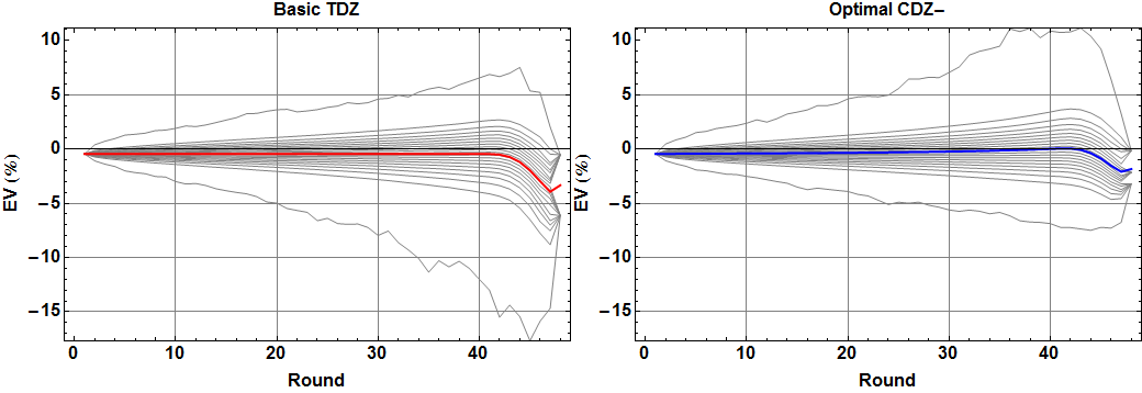
There are several interesting things happening here.  Let’s zoom in on just the red and blue curves indicating the mean EV per round:

Estimated expected value of a unit wager vs. round, for fixed basic TDZ strategy (red) and optimal CDZ- strategy (blue).

First, the red curve is nearly constant through most of the initial rounds of the shoe.  Actually, for every round that we are guaranteed to reach (i.e., not running out of cards before reaching the “cut-card” at 75% penetration), the true EV can be shown to be exactly constant.

Second, that extreme dip near the end of the shoe is illustration of the cut-card effect: if we manage to play an abnormally large number of rounds in a shoe, it’s because there were relatively few cards dealt per round, which means those rounds were rich in tens, which means that the remainder of the shoe is poor in tens, yielding a significantly lower EV.

Keep in mind that we can see this effect with less than 10 million total simulated rounds, with per-round EV estimates obtained from samples of at most 100,000 depleted shoe subsets!  This isn’t so surprising when we consider that each of those sample subsets indicates not just the net outcome of the round, but the exact expected outcome of the round, whose variance is much smaller… most of the time.  For the red TDZ and blue CDZ- strategies shown in the figure, there are actually three curves each, showing not just the estimated mean but also the (plus/minus) estimated standard deviation.  For the later rounds where the cut-card effect means that we have fewer than 100,000 sampled rounds, that standard deviation becomes large enough that we can see the uncertainty more clearly.

Variance

So far, none of this is really new; we have been able to efficiently compute basic and optimal strategy expected return for some time.  The interesting new data is the corresponding pre-deal variance (derived from the exact probability distribution).  The following figure shows an initial look at this, as a scatter plot of variance vs. EV for each round, with an overlaid smoothed histogram to more clearly show the density:

Variance vs. expected value of a unit wager, for fixed basic TDZ strategy (left) and optimal CDZ- strategy (right).

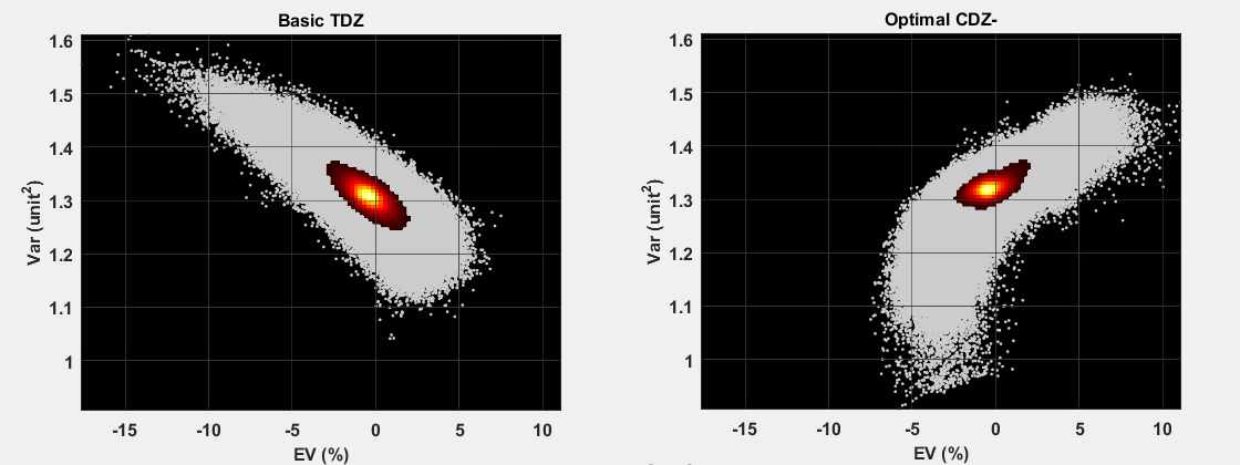
It seems interesting that the correlation sense is roughly reversed between basic and optimal strategy; that is, for the basic strategy player, higher EV generally means lower variance, while for the optimal strategy player with the laptop, the reverse is true.  I can’t say I anticipated this behavior, and upon first and second thoughts I still don’t have an intuitive explanation for what’s going on.