Probabilities in Knockout

Posted on October 31, 2014 by possiblywrong

Recently, my two youngest nephews have started playing basketball. Several weeks ago, I taught them– along with my wife– how to play Knockout, a game I remember playing at the various basketball camps I attended as a kid. The rules are pretty simple:

The $n$ players line up behind the free throw line, with the first two players each having a basketball. (At camp $n$ was often 80 or so, with the line stretching to the other end of the court, but in this case $n=4$ .) Each player in turn shoots initially from the free throw line. If he makes it, he passes the ball to the next player and goes to the end of the line. If he misses, he must recover the ball and shoot again– not necessarily from the free throw line– until he makes it. If a player ever fails to make a shot before the player behind him makes his shot, he is “knocked out” of the game. The last player remaining wins.

How fair is this game? That is, if we assume that all players are equally skilled, how important is your choice of starting position in line? Intuitively, it seems like it would be better to start nearer the end of the line, with the extent of advantage depending on the assumed difficulty of all shots taken. As usual, my intuition turned out to be wrong (or at least not entirely correct), which is why I think this is an interesting problem.

Let’s model the game by assuming that each player during his turn makes the initial free throw with probability $p$ , and (after a miss) makes any following shot with probability $q$ . (My guess at reasonable values for $p$ are somewhere between 0.4 and 0.6, with $q$ somewhere between 0.7 and 0.9.) Also, let’s assume that players always alternate shots, so that a player never gets two consecutive opportunities to make his shot without the other player shooting.

To make this more precise, the following figure shows the transitions between the five basic game states, with each node representing a shooting situation $s_i$ for the ordered subset of numbered players currently remaining in the game, with the player to shoot indicated in red.

Transitions between game states in Knockout. The numbered player to shoot is shown in red.

(For reference, a simplified two-player variant of this game was discussed earlier this year at Mind Your Decisions. However, that game is still not quite Knockout as discussed here, even restricting to $n=2$ players and $p=q$ . For example, if players 1 and 2 both miss, then player 1 makes his following shot, he does not immediately win the game.)

Knockout is relatively easy to simulate, but is a bit more challenging to approach analytically. Like the dice game Pig discussed earlier this year, the problem is that game states can repeat, so a straightforward recursive or dynamic programming solution won’t work.

So, as usual, to present the problem as a puzzle: in the game of Knockout with just $n=2$ players, as a function of $p$ and $q$ , what is the probability that the first player wins?

(Hint: I chose $n=2$ not just because it’s the simplest starting point, but because I think the answer is particularly interesting in that case: the probability does not depend on $q$ !)

Calories in, calories out

Posted on October 21, 2014 by possiblywrong

This article was discussed on Hacker News.

Introduction

How do we lose (or gain) weight? Is it really as simple as “calories in, calories out” (i.e., eat less than you burn), or is what you eat more important than how much? Is “3500 calories equals one pound” a useful rule of thumb, or just a myth? I don’t think I would normally find these to be terribly interesting questions, except for the fact that there seems to be a lot of conflicting, confusing, and at times downright misleading information out there. That can be frustrating, but I suppose it’s not surprising, since there is money to be made in weight loss programs– whether they are effective or not– particularly here in the United States.

Following is a description of my attempt to answer some of these questions, using a relatively simple mathematical model, in an experiment involving daily measurement of weight, caloric intake, and exercise over 75 days. The results suggest that you can not only measure, but predict future weight loss– or gain– with surprising accuracy. But they also raise some interesting open questions about how all this relates to the effectiveness of some currently popular diet programs.

(Edit 2017-08-11: When I originally posted this article 3 years ago, I quoted and linked to some sources whose calculations and/or arguments I disagreed with. One of those sources was professor of exercise science Gregory Hand, whose linked blog post has since been locked as private. Another was nutritionist Zoë Harcombe, whose linked blog post is still accessible, but has since been modified to no longer contain the argument as quoted here… but with a new “footnote” argument that indicates the same misunderstanding of the model described here. I’m leaving all of the original text and quotes here, but see below for an additional edit to comment on Harcombe’s footnote.)

The model and the experiment

Here was my basic idea: given just my measured starting weight $w_0$ , and a sequence $(c_n)$ of measurements of subsequent daily caloric intake, how accurately could I estimate my resulting final weight, weeks or even months later?

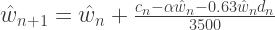
More precisely, consider the sequence $(\hat{w}_n)$ of predicted daily weights given by the following recurrence relation:

$\hat{w}_0 = w_0$

$\hat{w}_{n+1} = \hat{w}_n + \frac{c_n - \alpha \hat{w}_n - 0.63 \hat{w}_n d_n}{3500}$

Intuitively, my weight tomorrow morning $\hat{w}_{n+1}$ should be my weight this morning $\hat{w}_n$ , plus the effect of my net intake of calories that day, assuming 3500 calories per pound. Net calorie intake is modeled with three components:

$c_n$ is the number of calories consumed.
$-\alpha\hat{w}_n$ is the number of calories burned due to normal daily activity. Note that this is a function of current weight, with typical values for $\alpha$ of 12 to 13 calories per pound for men, or 10 to 11 for women; I used 12.5 (more on this later).
$-0.63 \hat{w}_n d_n$ is the number of additional calories burned while running (my favorite form of exercise), where $d_n$ is the number of miles run that day. Note that we don’t really have to account for exercise separately like this; especially if duration and intensity don’t change much over time, we could skip this term altogether and just roll up all daily activity into the (larger) value for $\alpha$ .

(Aside: I am intentionally sticking with U. S. customary units of pounds, miles, etc., to be consistent with much of the related literature.)

So, at the start of my experiment, my initial weight was $w_0=251.8$ pounds (for reference, I am a little over 6’4″ tall, 40-ish years old). Over each of the next 75 days, I recorded:

My actual weight $w_n$ , first thing in the morning after rolling out of bed, using a digital scale with a display resolution of 0.1 pound.
My total calories consumed for the day $c_n$ .
My running mileage for the day $d_n$ .

Plugging in $c_n$ and $d_n$ to the recurrence relation above, I computed the sequence of predicted weights $(\hat{w}_n)$ , and compared with the sequence of my actual weights $(w_n)$ .

Results

The following figure shows the resulting comparison of predicted weight $\hat{w}_n$ (in blue) with measured actual weight $w_n$ (in red). See the appendix at the end of this post for all of the raw data.

Predicted and actual weight over 75 days.

I was surprised at just how well this worked. Two and a half months and nearly 30 pounds later, the final predicted weight differed from the actual weight by less than a pound!

There are a couple of useful observations at this point. First, the “3500 calories per pound” rule of thumb is perfectly valid… as long as it is applied correctly. Zoë Harcombe, a “qualified nutritionist,” does a great job of demonstrating how to apply it incorrectly:

“Every person who didn’t have that [55-calorie] biscuit every day should have lost 141 pounds over the past 25 years.”

This seems to be a common argument– professor of exercise science Gregory Hand makes a similar but slightly more vivid claim using the same reasoning about a hypothetical dieter, that “if she will lose 1 lb for every 3,500 calorie deficit [my emphasis], our individual will completely disappear from the face of the earth in 300 days.”

The problem in both cases is the incorrect assumption that an initial calorie deficit, due to skipping a biscuit, for example, persists as the same deficit over time, causing a linear reduction in weight. But that’s not how it works: as weight decreases, calorie expenditure also decreases, so that an initial reduced diet, continued over time, causes an asymptotic reduction in weight. (In the context of the recurrence relation above, Harcombe and Hand’s calculation effectively replaces the varying $\alpha \hat{w}_n$ in the numerator with the constant $\alpha w_0$ .)

(Edit 2017-08-11: Harcombe’s blog post no longer contains the above quote, but has since been edited to include the following footnote:

“If we think one pound equals 3,500 calories and in fact one pound equals 2,843 calories, over a year, 657 ‘extra’ calories a day, simply from the formula ‘being wrong’, would add up to 239,805 extra calories and this, divided by 2,843 gives 84 pounds, or six stone. Adjust the calculations for women more typically maintaining at 2,000 calories a day and men more typically at 2,600 calories a day and the inaccuracy of the formula still creates wide disparity.”

This argument still exhibits the same problem. It is unclear how we should interpret the calculation of 84 pounds; the word “extra” seems to suggest the idea that a person whose diet was structured assuming an incorrect 3500 calories per pound (when the “real” value is 2843) would… what? Gain 84 pounds over the course of a year? If anything, I would expect to lose more weight if the “cost” of losing each pound of fat was burning fewer calories.

But even ignoring the sign issue, the real problem as mentioned above is not the accuracy of choice of denominator in the division, but the fixed numerator. To see why, consider the example of an overweight man who weighs 250 pounds, burns 12.5 calories per pound per day, and plans to eat 2600 calories per day for the next year. Using the recurrence relation described here, assuming “3500 calories per pound,” he expects to lose a little over 30 pounds in that year. If the correct value were really 2843 calories per pound, then his predicted final weight changes by… less than 3 pounds, over the course of an entire year.)

Estimating $\alpha$

The second– and, I think, most important– observation is that I arguably “got lucky” with my initial choice of $\alpha=12.5$ calories burned per pound of body weight. If I had instead chosen 12, or 13, the resulting predictions would not agree nearly as well. And your value of $\alpha$ is likely not 12.5, but something different. This seems to be one of the stronger common arguments against calorie-counting: even if you go to the trouble of religiously measuring calories in, you can never know calories out exactly, so why bother?

The Harris-Benedict equation is often used in an attempt to remedy this, by incorporating not only weight, but also height, age, gender, and activity level into a more complex calculation to estimate total daily calorie expenditure. But I think the problem with this approach is that the more complex formula is merely a regression fit of a population of varying individuals, none of whom are you. That is, even two different people of exactly the same weight, height, age, gender, and activity level do not necessarily burn calories at the same rate.

But even if you don’t know your personal value of $\alpha$ ahead of time, you can estimate it, by measuring calories in $(c_n)$ and actual weight $(w_n)$ for a few weeks, and then finding the corresponding $\alpha$ that yields a sequence of predicted weights $(\hat{w}_n)$ that best fits the actual weights over that same time period, in a least-squares sense.

The following figure shows how this works: as time progresses along the x-axis, and we collect more and more data points, the y-axis indicates the corresponding best estimate of $\alpha$ so far.

Estimating burn rate (alpha) over time. Early estimates are overwhelmed by the noisy weight measurements.

Here we can see the effect of the noisiness of the measured actual weights; it can take several weeks just to get a reasonably settled estimate. But keep in mind that we don’t necessarily need to be trying to lose weight during this time. This estimation approach should still work just as well whether we are losing, maintaining, or even gaining weight. But once we have a reasonably accurate “personal” value for $\alpha$ , then we can predict future weight changes assuming any particular planned diet and exercise schedule.

(One final note: recall the constant 0.63 multiplier in the calculation of calories burned per mile run. I had hoped that I could estimate this value as well using the same approach… but the measured weights turned out to be simply too noisy. That is, the variability in the weights outweighs the relatively small contribution of running to the weight loss on any given day.)

Edit: In response to several requests for a more detailed description of a procedure for estimating $\alpha$ , I put together a simple Excel spreadsheet demonstrating how it works. It is already populated with the time series of my recorded weight, calories, and miles from this experiment (see the Appendix below) as an example data set.

Given a particular calories/pound value for $\alpha$ , you can see the resulting sequence of predicted weights, as well as the sum of squared differences (SSE) between these predictions and the corresponding actual measured weights.

Or you can estimate $\alpha$ by minimizing SSE. This can either be done “manually” by simply experimenting with different values of $\alpha$ (12.0 is a good starting point) and observing the resulting SSE, trying to make it as small as possible; or automatically using the Excel Solver Add-In. The following figure shows the Solver dialog in Excel 2010 with the appropriate settings.

Excel Solver dialog showing the desired settings to estimate alpha minimizing SSE.

Conclusions and open questions

I learned several interesting things from this experiment. I learned that it is really hard to accurately measure calories consumed, even if you are trying. (Look at the box and think about this the next time you pour a bowl of cereal, for example.) I learned that a chicken thigh loses over 40% of its weight from grilling. And I learned that, somewhat sadly, mathematical curiosity can be an even greater motivation than self-interest in personal health.

A couple of questions occur to me. First, how robust is this sort of prediction to abrupt changes in diet and/or exercise? That is, if you suddenly start eating 2500 calories a day when you usually eat 2000, what happens? What about larger, more radical changes? I am continuing to collect data in an attempt to answer this, so far with positive results.

Also, how much does the burn rate $\alpha$ vary over the population… and even more interesting, how much control does an individual have over changing his or her own value of $\alpha$ ? For example, I intentionally paid zero attention to the composition of fat, carbohydrates, and protein in the calories that I consumed during this experiment. I ate cereal, eggs, sausage, toast, tuna, steak (tenderloins and ribeyes), cheeseburgers, peanut butter, bananas, pizza, ice cream, chicken, turkey, crab cakes, etc. There is even one Chipotle burrito in there.

But what if I ate a strict low-carbohydrate, high-fat “keto” diet, for example? Would this have the effect of increasing $\alpha$ , so that even for the same amount of calories consumed, I would lose more weight than if my diet were more balanced? Or is it simply hard to choke down that much meat and butter, so that I would tend to decrease $c_n$ , without any effect on $\alpha$ , but with the same end result? These are interesting questions, and it would be useful to see experiments similar to this one to answer them. (Edit: See this later post for a follow-up with an additional two months of recorded data.)

Appendix: Data collection

The following table shows my measured actual weight in pounds over the course of the experiment:

Mon     Tue     Wed     Thu     Fri     Sat     Sun
251.8   251.6   250.6   249.8   248.4   249.8   249.0
250.4   249.0   247.8   246.6   246.6   247.8   246.2
246.6   244.0   244.6   243.6   243.6   244.0   244.8
242.0   240.6   240.4   240.2   240.2   239.4   238.6
238.0   238.0   237.6   238.0   238.0   238.6   238.6
237.4   239.0   237.6   235.8   236.0   235.0   236.0
233.8   232.4   232.6   233.4   233.4   232.0   233.2
232.6   231.6   232.2   232.2   231.2   231.2   229.6
229.6   229.6   230.6   230.4   229.8   228.0   227.4
227.6   226.2   226.4   225.6   225.8   225.8   226.0
228.0   225.8   225.4   224.6   223.8

The following table shows my daily calorie intake:

Mon     Tue     Wed     Thu     Fri     Sat     Sun
1630    1730    1670    1640    2110    2240    1980
1630    1560    1690    1700    2010    1990    2030
1620    1710    1590    1710    2180    2620    2100
1580    1610    1610    1620    1690    2080    1930
1620    1680    1610    1610    1810    2550    2430
1710    1660    1630    1710    1930    2470    1970
1660    1750    1710    1740    2020    2680    2100
1740    1750    1750    1610    1990    2290    1940
1950    1700    1730    1640    1820    2230    2280
1740    1760    1780    1650    1900    2470    1910
1570    1740    1740    1750

And finally, the following table shows the number of miles run on each day:

Mon     Tue     Wed     Thu     Fri     Sat     Sun
2.5     0.0     2.5     0.0     0.0     2.5     0.0
2.5     0.0     2.5     0.0     0.0     2.5     0.0
2.5     0.0     2.5     0.0     0.0     3.0     0.0
2.5     0.0     2.5     0.0     0.0     3.0     0.0
2.5     0.0     3.0     0.0     0.0     3.0     0.0
2.5     0.0     3.0     0.0     0.0     3.0     0.0
3.0     0.0     3.0     0.0     0.0     3.0     0.0
3.0     0.0     3.0     0.0     0.0     3.0     0.0
3.0     0.0     3.0     0.0     0.0     3.5     0.0
3.0     0.0     3.0     0.0     0.0     3.5     0.0
3.0     0.0     3.5     0.0

No, diversity does not generally trump ability

Posted on October 9, 2014 by possiblywrong

I am pretty sure that my motivation for this post is simply sufficient annoyance. I admittedly have a rather harsh view of social “science” in general. But this particular study seems to have enough visibility and momentum that I think it’s worth calling attention to a recent rebuttal. Where by “rebuttal” I mean “brutal takedown.”

At issue is a claim by Lu Hong and Scott Page, including empirical evidence from computer simulation and even a mathematical “proof,” that “diversity trumps ability.” The idea is that when comparing performance of groups of agents working together to solve a problem, groups selected randomly from a “diverse” pool of agents of varying ability can perform better than groups comprised solely of the “best” individuals.

“Diversity” is a fun word. It’s a magnet for controversy, particularly when, as in this case, it is conveniently poorly defined. But the notion that diversity might actually provably yield better results is certainly tantalizing, and is worth a close look.

Unfortunately, upon such closer inspection, Abigail Thompson in the recent AMS Notices shows that not only is the mathematics in the paper incorrect, but even when reasonably corrected, the result is essentially just a tautology, with little if any actual “real world” interpretation or application. And the computer simulation, that ostensibly provides backing empirical evidence, ends up having no relevance to the accompanying mathematical theorem.

The result is that Hong and Page’s central claim enjoys none of the rigorous mathematical justification that distinguished it from most of the literature on diversity research in the first place. And this is what annoys me: trying to make an overly simple-to-state claim– that is tenuous to begin with– about incredibly complex human behavior, and dressing it up with impressive-sounding mathematics. Which turns out to be wrong.

References:

1. Hong, L. and Page, S., Groups of diverse problem solvers can outperform groups of high-ability problem solvers, Proc. Nat. Acad. of Sciences, 101(46) 2004 [PDF]

2. Thompson, Abigail, Does Diversity Trump Ability? An Example of the Misuse of Mathematics in the Social Sciences, Notices of the AMS, 61(9) 2014, p. 1024-1030 [PDF]

The discreet hotel manager

Posted on October 5, 2014 by possiblywrong

The following puzzle deals with storage and search strategies for querying membership of elements in a table. Like the light bulb puzzle, it’s an example of a situation where binary search is only optimal in the limiting case. I will try to present the problem in the same weirdly racy context in which I first encountered it:

You are the manager of a hotel that, once a year, hosts members of a secretive private club in $n=10$ numbered suites on a dedicated floor of the hotel. There are $m=18$ club members, known to you only by numbers 1 through $m$ . Each year, some subset of 10 of the 18 club members come to the hotel for a weekend, each staying in his own suite. To preserve secrecy, you assign each man to a suite… but then destroy your records, including the list of the particular members staying that weekend.

It may be necessary to determine whether a particular member is staying at the hotel (say, upon receiving a call from his wife asking if her husband is there). But the club has asked that in such cases you must only knock on the door of a single suite to find out who is residing there. For a given subset of 10 club members, how should you assign them to suites, and what is your “single-query” search strategy for determining whether any given club member is staying at your hotel?

This problem is interesting because, for a sufficiently large universe $m$ of possible key values, we can minimize the maximum number of queries needed in a table of size $n$ by storing the $n$ keys in sorted order, and using binary search, requiring $\lceil lg(n+1) \rceil$ queries in the worst case. But for small $m$ , as in this problem, we can do better. For example, if $m=n$ , then we don’t need any queries, since every key is always in the table. If $m=n+1$ , then we can store in a designated position the key immediately preceding (cyclically if necessary) the missing one, requiring just a single query to determine membership.

(Hint: The problem is setup to realize a known tight bound: if $m \leq 2(n-1)$ , then there is a strategy requiring just a single query in the worst case.)

Possibly Wrong

On science, mathematics, and computing

Monthly Archives: October 2014

Probabilities in Knockout

Calories in, calories out

No, diversity does not generally trump ability

The discreet hotel manager