September | 2015 | Possibly Wrong

Introduction

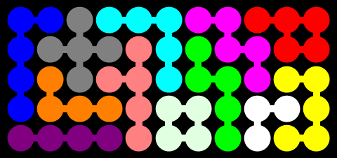
During a recent vacation flight, my nephews had a couple of interesting puzzles to occupy them on the plane: Kanoodle and IQ Fit. In both cases, the objective is to arrange a set of colored pieces so that they exactly fill a rectangular grid, as in the following figure showing an example solution to the Kanoodle puzzle:

Example solution to Kanoodle puzzle.

The IQ Fit version uses a smaller 5-by-10 grid, and only 10 pieces instead of 12… but the pieces are three-dimensional, so that some of the spherical “vertices” of the pieces may poke down through the bottom of the tray. (For reference, following is Python code specifying the configurations of pieces for both puzzles.)

kanoodle = {
    'Green': ((1, 1, 0), (1, 2, 0), (2, 2, 0), (2, 3, 0), (2, 4, 0)),
    'Cyan': ((1, 1, 0), (1, 2, 0), (1, 3, 0), (2, 3, 0), (3, 3, 0)),
    'Purple': ((1, 1, 0), (1, 2, 0), (1, 3, 0), (1, 4, 0)),
    'Yellow': ((1, 1, 0), (1, 2, 0), (2, 2, 0), (3, 1, 0), (3, 2, 0)),
    'Orange': ((1, 1, 0), (2, 1, 0), (2, 2, 0), (2, 3, 0)),
    'Blue': ((1, 2, 0), (2, 2, 0), (3, 2, 0), (4, 1, 0), (4, 2, 0)),
    'Pink': ((1, 1, 0), (1, 2, 0), (1, 3, 0), (1, 4, 0), (2, 3, 0)),
    'Gray': ((1, 2, 0), (2, 1, 0), (2, 2, 0), (2, 3, 0), (3, 2, 0)),
    'Magenta': ((1, 1, 0), (1, 2, 0), (2, 2, 0), (2, 3, 0), (3, 3, 0)),
    'Red': ((1, 1, 0), (1, 2, 0), (2, 1, 0), (2, 2, 0), (2, 3, 0)),
    'White': ((1, 1, 0), (2, 1, 0), (2, 2, 0)),
    'LightGreen': ((1, 1, 0), (1, 2, 0), (2, 1, 0), (2, 2, 0))
    }

iq_fit = {
    'Green': ((1, 1, 0), (2, 1, 0), (2, 2, 0), (3, 1, 0),
              (1, 1, -1), (2, 1, -1)),
    'Magenta': ((1, 1, 0), (1, 2, 0), (1, 3, 0), (2, 2, 0),
                (2, 3, 0), (1, 1, -1)),
    'Cyan': ((1, 1, 0), (1, 2, 0), (1, 3, 0), (1, 4, 0),
             (2, 2, 0), (1, 2, -1), (1, 3, -1)),
    'LightGreen': ((1, 1, 0), (1, 2, 0), (2, 2, 0), (3, 1, 0),
                   (3, 2, 0), (3, 2, -1)),
    'Blue': ((1, 4, 0), (2, 1, 0), (2, 2, 0), (2, 3, 0), (2, 4, 0),
             (2, 2, -1), (2, 4, -1)),
    'Purple': ((1, 1, 0), (1, 2, 0), (1, 3, 0), (2, 2, 0),
               (1, 1, -1), (1, 3, -1)),
    'Yellow': ((1, 1, 0), (1, 2, 0), (2, 1, 0), (2, 2, 0), (2, 3, 0),
               (2, 4, 0), (2, 4, -1)),
    'Pink': ((1, 1, 0), (1, 2, 0), (1, 3, 0), (1, 4, 0), (2, 1, 0),
             (2, 2, 0), (1, 2, -1)),
    'Orange': ((1, 3, 0), (2, 1, 0), (2, 2, 0), (2, 3, 0), (2, 4, 0),
               (2, 1, -1), (2, 3, -1)),
    'Red': ((1, 4, 0), (2, 1, 0), (2, 2, 0), (2, 3, 0), (2, 4, 0),
            (2, 1, -1), (2, 4, -1))
    }

A natural question to ask is: which puzzle is harder? For example, which puzzle has more possible solution configurations? Can we count them all? It turns out that we can, using Donald Knuth’s “Dancing Links” (DLX) algorithm (see references below). But the motivation for this post is to describe another interesting application of DLX: before attempting an exact count, we can first estimate the number of solutions, to determine whether it is even worth trying to enumerate them.

Exact Cover

The Kanoodle and IQ Fit puzzles are examples of the more general exact cover problem: given a matrix of 0s and 1s, does it have a set of rows containing exactly one 1 in each column? Many other problems may also be reduced to that of finding an exact cover: Sudoku, Langford sequences, and graph colorings are just a few examples.

Often the most interesting part of solving many of these problems is figuring out the transformation to an exact cover instance. That is, how do we construct a 0-1 matrix representing our problem, so that a set of rows containing exactly one 1 in each column corresponds to a solution to our problem? In the case of Kanoodle (and IQ Fit is similar), there are two “kinds” of columns: one column for each of the 12 puzzle pieces, and one column for each position in the 5-by-11 rectangular grid. Each row of the matrix represents a possible placement of one of the pieces, with a single 1 in the corresponding “piece” column, and additional 1s in the corresponding occupied “position” columns. A set of rows solving the exact cover problem will have exactly one row for each piece, oriented and positioned so that all of the grid positions are occupied by exactly one piece.

Considering all possible placements of all pieces, the Kanoodle puzzle has a total of 1789 rows and 67 columns, while the IQ Fit puzzle has 3440 rows and 60 columns. (David Austin wrote a great AMS Feature Column on this same topic, suggesting that the Kanoodle puzzle has 2222 rows; there are a couple of bugs in his implementation, however, yielding some extra invalid piece placements and some missing valid ones.)

Dancing Links (DLX)

Now that we have a matrix representing our exact cover problem, we can feed it to Knuth’s Dancing Links algorithm (referred to as DLX), which is essentially “just” a backtracking depth-first tree search for all possible solutions, but with a “doubly-doubly” linked list sparse matrix representation that allows very efficient undo operations. I won’t bother with details here, especially since Knuth’s paper is so readable.

My implementation is available in the usual location here, as well as on GitHub. There isn’t much there; the search algorithm itself follows Knuth’s pseudocode nearly verbatim, right down to the variable names.

There are quite a few DLX implementations in the wild already, but I ended up writing my own for several reasons. First, the matrix row and column identifiers should be of generic types; the “real” problem is rarely represented in terms of simple consecutive integer matrix indices. Second, it seemed reasonable to be able to construct the sparse matrix by adding 1s individually, in any order. Although the diagrams in Knuth’s paper suggest a nice “weaving loom” look to the data structure, there is no need to preserve any particular order relation on the rows or columns. Third, although I didn’t use it for this analysis, it was relatively simple to add support for “secondary,” or optional columns, which must be covered at most once, instead of exactly once. (As discussed in Knuth’s paper, the N queens problem is a natural example where this is handy.)

Estimating Tree Size

Finally, and most importantly, I wanted to try using the Monte Carlo sampling technique, mentioned briefly in Knuth’s DLX paper, to estimate the size of the search tree without actually exploring all of it. As Knuth puts it (see Reference (3) below):

Sometimes a backtrack program will run to completion in less than a second, while other applications seem to go on forever. The author once waited all night for the output from such a program, only to discover that the answers would not be forthcoming for about 1,000,000 centuries.

The sampling algorithm is pretty simple: take a random walk from the root of the tree to a leaf, at each step recording the (out-)degree $d_k$ of the current vertex at depth $k$ , and selecting a child vertex (at depth $k+1$ ) uniformly at random. It is not difficult to show by induction that the expected value of the resulting product of degrees along the sample path equals the total number of leaves in the tree.

Furthermore, the expected value of the product $d_0 d_1 d_2 ... d_{k-1}$ for some fixed $k$ equals the total number of vertices at depth $k$ in the tree… as long as we define $d_j=0$ for depths $j$ beyond the length of the (possibly shorter) sample path.

This algorithm almost feels like cheating; we are trying to estimate the size of an entire tree, when there are whole chunks of it that we may never explore!

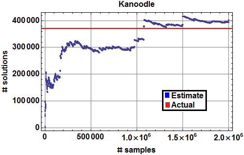
The following figure shows the result of 2 million such random paths through the Kanoodle DLX search tree. The blue points indicate the current running estimate of the total number of solutions– more precisely, the number of tree vertices at depth 12.

Monte Carlo estimate of number of Kanoodle solutions (blue), with actual number of solutions (red).

In this case, the couple of minutes needed to collect the random samples turned out to be longer than the 30 seconds to simply traverse the entire tree, yielding exactly 371,020 different solutions to the Kanoodle puzzle (shown in red above).

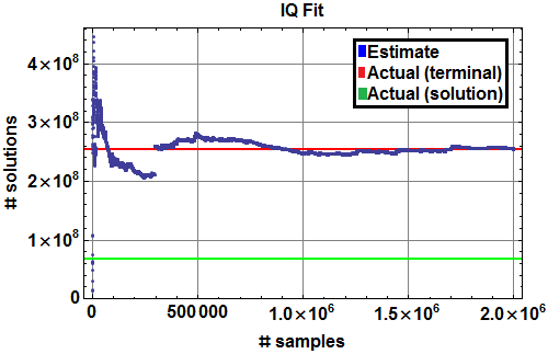
The IQ Fit puzzle was more interesting; the following figure again shows the running estimate (in blue) of the number of leaf vertices at depth 10 in the DLX search tree.

Monte Carlo estimate of number of IQ Fit solutions (blue), with actual number of depth 10 terminal vertices (red), and actual number of solutions (green).

Using this estimate of what turned out to be exactly 254,531,140 vertices at depth 10 (shown in red above), I expected to get an exact count via a full tree traversal in about 6 hours. However, just an hour and a half later, my program had already stopped, reporting that there were only 67,868,848 solutions (shown in green), about one-fourth what I expected. What was going on?

After further investigation, I realized that, unlike the Kanoodle puzzle, it is possible to arrange the three-dimensional IQ Fit pieces so that all 10 pieces fit into the grid… but with some spaces still left unfilled. These non-solution arrangements account for the remaining three-fourths of the leaf vertices at depth 10 in the tree.

References:

Austin, D., Puzzling Over Exact Cover Problems, American Mathematical Society Feature Column, December 2009 (HTML)
Knuth, D., Dancing Links, Millenial Perspectives in Computer Science, 2000, p. 187-214 (arXiv)
Knuth, D., Estimating the efficiency of backtrack programs, Mathematics of Computation, 29 (1975), p. 121–136 (PDF)

This is to capture notes on my progress toward a solution to the “matching quiz” problem presented in the previous post, which can be re-stated more concisely as follows: what is the optimal strategy for choosing quiz answers specified as a function $f : [n] \rightarrow [n]$ , not necessarily a bijection, that maximizes the probability of agreeing with a randomly chosen “solution” bijection in at least $m$ questions?

A strategy is characterized by a partition $\lambda$ of $n$ , with the parts corresponding to the sizes of the classes of the equivalence kernel of the chosen function $f$ . The number of parts in the partition indicates the number of distinct quiz answers. For example,

$1 + 1 + ... + 1 = n$

corresponds to a bijection, and the single-part partition $n=n$ corresponds to a constant function, i.e., writing the same answer for all $n$ questions. Note that any function with the same partition “signature” has the same probability of success.

So, given a guessing strategy specified as a partition with $k$ parts:

$\lambda = \lambda_1 + \lambda_2 + ... + \lambda_k = n$

what is the probability of getting at least $m$ answers correct? First, we can compute the probability $p(S)$ that exactly some subset $S \subseteq [k]$ of distinct answers is correct using inclusion-exclusion:

$p(S) = \frac{1}{n!} \sum\limits_{T \supseteq S} (-1)^{|T|-|S|}(n-|T|)! \prod\limits_{i \in T} \lambda_i$

And so the overall probability of at least $m$ correct answers is

$P(success) = \sum\limits_{|S| \geq m} p(S)$

We can collapse this sum of sums by observing that a particular subset $T \subseteq [k]$ in the inner summation appears ${|T| \choose |S|}$ times in the outer summation for a given size $|S|$ . Using the identity

$\sum\limits_{s=m}^t (-1)^{t-s} {t \choose s} = (-1)^{t-m} \frac{m}{t} {t \choose m}$

we can compute the overall probability of at least $m$ correct answers as

$P(success) = \frac{1}{n!} \sum\limits_{|T| \geq m} (-1)^{|T|-m} \frac{m}{|T|} {|T| \choose m} (n-|T|)! \prod\limits_{i \in T} \lambda_i$

At this point, I’m stuck; I don’t see a better approach than simply evaluating all possible strategies (i.e., generating all integer partitions of $n$ ) for small values of $1 \leq m \leq n$ , and looking for patterns. Following is the conjectured optimal strategy which holds for $n \leq 16$ :

If $m=1$ , then as pointed out in the previous post, write down the same answer $n$ times, guaranteeing exactly one correct answer.
For $m=2$ , write one answer $\lfloor n/2 \rfloor$ times, and another (different) answer $\lceil n/2 \rceil$ times.
For $m=n-1$ , select an “almost-permutation,” corresponding to the integer partition $1+1+...+1+2=n$ , so that exactly one answer gets duplicated (and thus exactly one answer is missing).
Otherwise, select a random permutation.

Actually, we can describe this strategy more efficiently as follows: (a) select $m$ distinct answers, and distribute them as evenly as possible among the $n$ questions… unless $2<m<n-1$ , in which case (b) just select a random permutation. I think (a) is what intuition would suggest is always the optimal approach– it was my wife’s immediate response when I described the problem to her– but I don’t have a good explanation for the qualification (b).

Possibly Wrong

On science, mathematics, and computing

Monthly Archives: September 2015

Kanoodle, IQ Fit, and Dancing Links

The clueless student: solution